Design S3 Object Storage.
Object Storage Service - Amazon Simple Storage Service S3.
The service provide by AWS that provide object storage through a RESTful API based interface.
2006: 🚀 S3 launched.
2010–2011: 🔐 Key features added — versioning, bucket policy, multipart upload support, encryption, multiobject delete, object expiration.
2013: 📦 2 trillion objects milestone.
2014–2015: 🔁 Lifecycle, notifications, cross-region replication.
2021: 💥 100 trillion objects stored.
Storage System Understanding
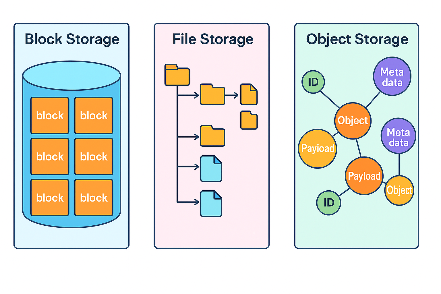
Storage system falls in 3 broad categories - Block storage, File storage, Object storage.
Block Storage.
In 1960s, common devices like Hard Disk Drive and Solid State Drive that are physically atatched to the server.
Block storage can be connected over high speed network using Fibre Channel FC and iSCSI.
It presents a raw block to the server as volumes. Raw block - unstructured form of data. Combined together form a volume which is container that the server can use.
The flexible and versatile form of storage and can be used by server as file system or anything.
🧠 Quick Mnemonic: “RAW = Ready, Adaptable, Writable” Ready for formatting or direct use
Adaptable to different workloads
Writable by server or application logic.
File Storage.
Build on top of block storage and provide a ligher level of abstraction to easy the file and directories.
File storage could be made accessible by a large number of servers using common file level network protocols like SMB/CIFS and NFS.
The most easy way to manage the storage. The server accessing fiel storage so not need to deal with teh complexity of managing the blocks, formatting volumes.
Object Storage.
Object stirage stores all data as object in a flat structure. No hierarchical directory structure. Data access is normally providede by RESTful APIs.
Object stirage makes a tradeoff to high durability, vast scale and low cost.
It target cold data ns mainly used for archival and backup.
Slow compared to other storage type.
Example - AWS S3, Google Object Storage, Azure Blob Stirage.
Comparison
| Topic | Block Storage | File Storage | Object Storage |
|---|---|---|---|
| Update Content | Y | Y | N(object versioning possible but no in-place update). |
| Cost | High | Medium | Low |
| Performance | Medium to high, very high | Medium to high. | Low to Medium. |
| Data Access | SAS/iSCSI/FC | Standard file access CIFS/SMB and NFS. | RESTful API. |
| Scalability | Medium Scalability. | High Scalability. | Vast Scalability. |
| Application | VM, high performance application like database. | General purpose. | Binary data, Unstructured data. |
Object Storage Understanding.
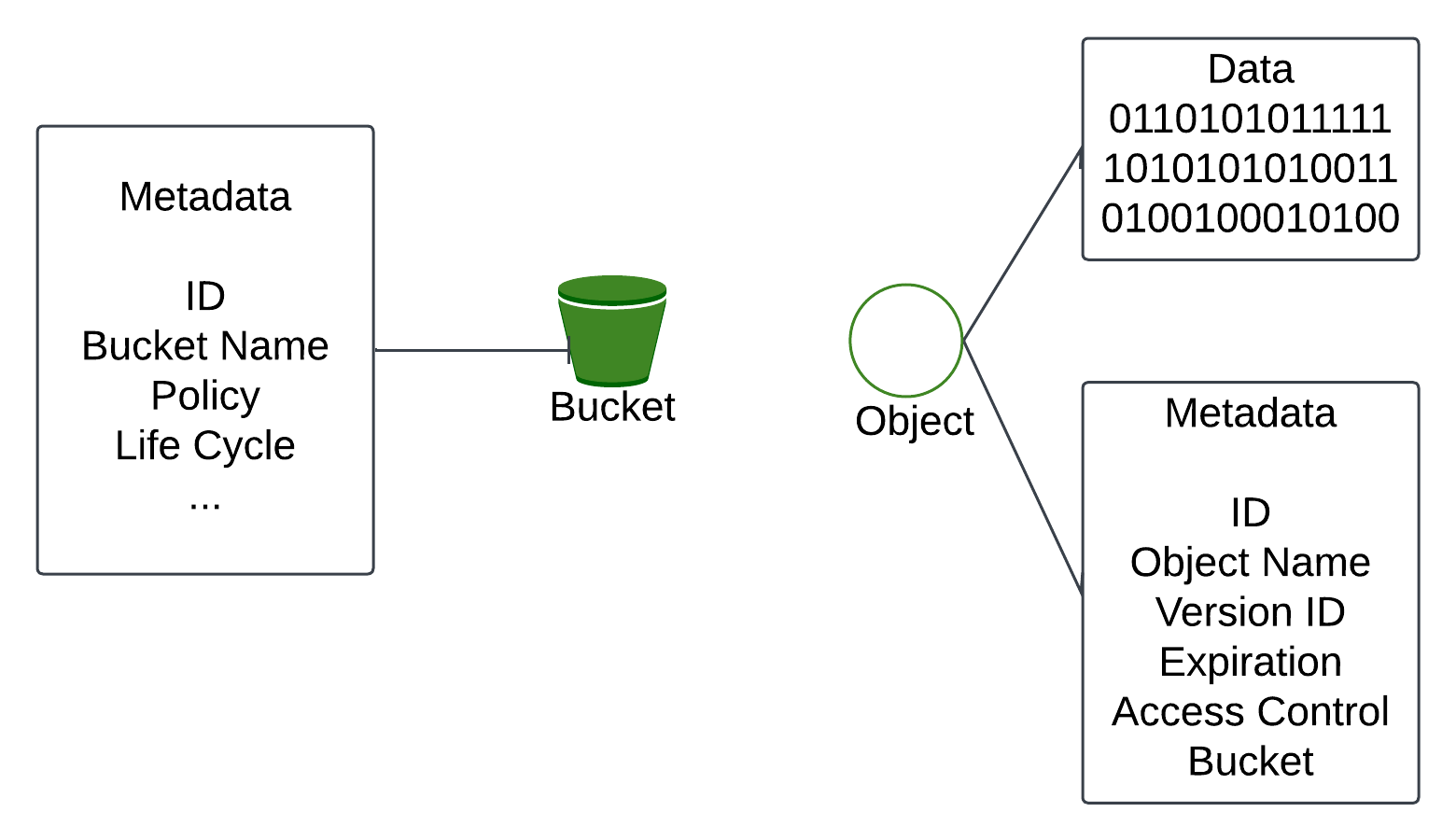
Bucket - A logical container for objects. It is globally unique. To upload data in S3 first create a bucket.
Object.
Object is an individual piece of data we store in the bucket. It contain object data called payload and metadata. Object data can be any sequence of byte and the metadata is the set of name-value pairs that describe the object.
Versioning.
A feature that keeps multiple variants of an object in the same bucket. Enabled at bucket level and user can recover objects.
Uniform Resource Identifier URI.
The object storage provides RESTful API to access its resource like bucket and objects. Each resource is identified by its URI.
Service Level Agreement SLA.
A SLA is a contract provided by the service provider and client. Example - S3 Standard-Infrequent Access stirage class provides the SLA - DEsigned for durability of 99. 11 nines of objects across multiple availability zones. Data is resilient in the evnt of oe entire availability zone destruction. Designed for 99.9% availability.
Understand the problem.
What features included in the design?
Bucket creation, Object uploading and downloading, Object versioning, listing objects in a bucket like the aws S3 ls command.
Data size - Need to store massive object like GBs and a large number of small object like KBs.
Data we need to store one year - 100 PB.
Data durability of 6 nines (99.9999%) and service availability of 4 nines (99.99%).
Non Functional Requirements.
100PB of data. Data durability of 6 nines and service availability of 4 nines.
Storage Efficiency - Reduce storage costs while maintaining a high degree of reliability and performance.
Back of the envelope Estimation.
Object storge bottleneck in either disk capacity or disk IO per second IOPS.
Disk capacity - Example - 20% of all objects are small object(less than 1MB). 60% of objects are medium-sized objects(1Mb ~ 64MB). 20% are large objects(larger than 64MB).
IOPS - Example Hard disk (SATA interface 7200 rpm) is capable of doing 100 ~ 150 random seeks per second (100 ~ 150 IOPS).
We can estimate the total number of objects the system can persist. The median size for each object type (0.5MB for small object, 32MB for medium object and 200MB for large object). A 40% storage usage ratio - 100PB = 10010001000*1000 MB = 10^11 MB.
= (10^11 * 0.4)/(0.20.5 MB + 0.632MB + 0.2*200 MB) = 0.68 billion objects.
Metadata is 1Kb in size we need 0.68TB space to store all metadata information.
High Level Design.
Important properties of the object storage.

Object Immutability - One of the main difference between object storage and other storage is the object stores in object storage are immutable. WE can delete or replace them with new version - no incremental change.
Key-Value Store - We can use Object URI to get object data. Object URI is the key and the object data is the value.
Request - GET /bucket/object1.txt HTTP/1.1
Response - HTTP/1.1 200 OK Content-length: 4567
[4567 bytes of object data]
Write Once and read many times.
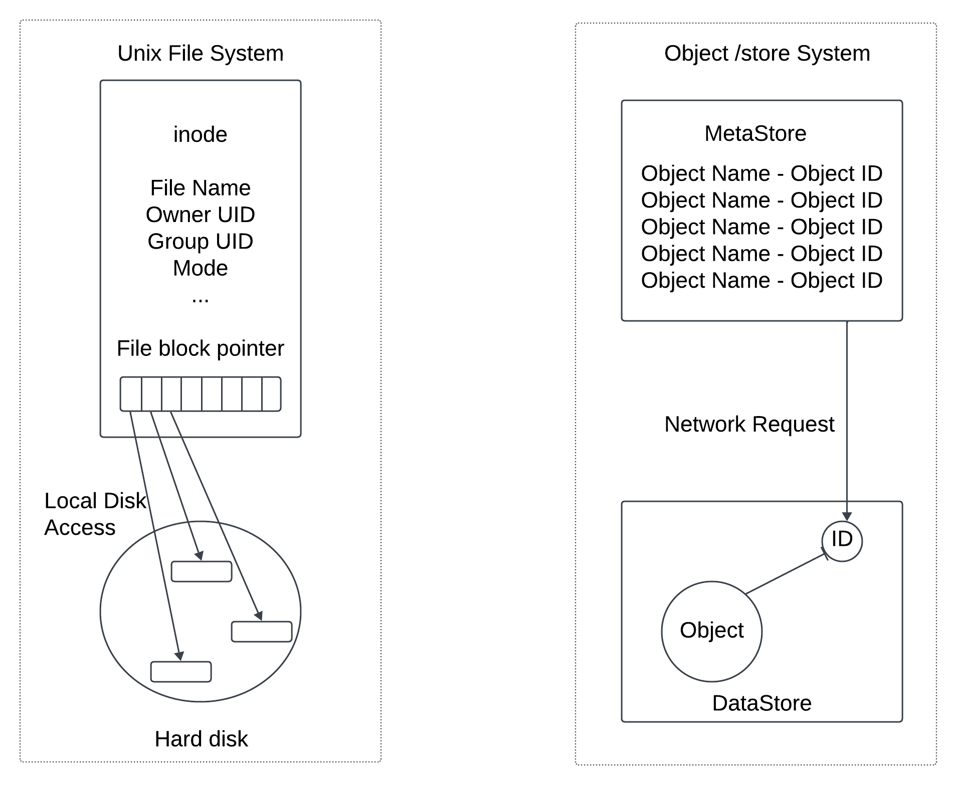
Support both small and large objects - The design philosophy of objects storage is very similar to UNIX file system when we save the file in the local storage it does not save the filename and file data together. Instead the filename is stored in a data structure called inode the file data is stored in different disk location.
inode contain a list of file block pointers that point to the disk locations of the file data. When we access a local file we first fetch the metadata in the inode then read the file data following the file block pointers to the actual disk location.
The object storage works in same way inode become the metadata store storing all objects. The hard disk become the data store that stores the object data. In UNIX file system the inode uses the file block pointer to record the location of data on the hard disk.
IN object storage the metadata store uses the ID of the object to find the object data in the data store via a network request.
The data store contains the immutable data and the metadata store contains the mutable data.
The separation enables us to implement and optimize these two components independently.
High Level Image - HighLevelDesign present.
Load Balancer - Distribute the load to the API servers.
API Services - Orchestrates remote procedure calls to the identity and access management service, metadata service and storage stores. The service is stateless so it can be horizontally scaled.
Identity and Access Management IAM - The central place to handle authentication, authorization and access control. Authentication verifies who you are and authorization validates what operations you could perform based on who you are.
Data store - Stores and retrieves the actual data. All data-related operations are based on object ID UUID.
Metadata store - Stores the metadata of the objects.
Uploading an Object.
In the high level design, first create a bucket names bucket-to-share and then upload a file name script.txt to the bucket.
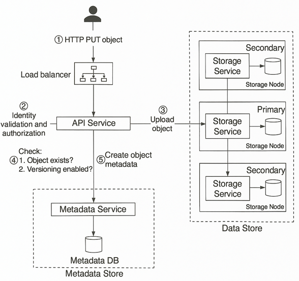
Client send the HTTP PUT requests to create a bucket names bucket-to-share. The request is forwarded to the API service. The SPI service calls the IAM to ensure the user is authorized and has the WRITE permission.
The API service calls the metadata store to create an entry with the bucket info in the metadata database. Once the entry is created the success message is returned to the client. Bucket create then the client sends an HTTP PUT request to create an object names script.txt. The API service verifies the users identity and ensures the user has the WRITE permission.
The validation succeeds the API service sends the object data in the HTTP PUT payload to the data store. The data store persists the payload as an object and returns the UUID of the object.
The API service calls the metadata store to create a new entry in the metadata database. It contains imp metadata such as the object_id, bucket_id, object_name.
API to upload an object.
PUT /bucket-to-share/script.txt HTTP/1.1
Host - foo.s3example.org
Date - Sun, 24 Sept 2025 19:30:00 GMT
Authorization - Authorization String
Content-Type - text/plain
Content-length - 4567
author - Rohan

[4567 bytes of object data]
Downloading an Object.
A bucket has no directory hierarchy. We can create a logical hierarchy by concatenating the bucket name and the object name to get a folder structure. Example bucket-to-share/script.txt To get an object we specify the object name in the GET request.
API to download an object.
GET /bucket-to-share/script.txt HTTP/1.1
Host - foo.s3example.org
Date - Sun, 29 Sept 2025 23:30:00 GMT
Authorization - Authorization String
The data store does not store the name of the object and it only supports object operations using the object_id(UUID). To download the object first map the object name to the UUID.
The client sends a GET request to the loadbalancer. The API service queries the IAM to verify the user has READ access. Once validated the API service fetches the UUID from the metadata store.
The API service fetches the object data from the data store by its UUID. It return the object data to the client in HTTP GET response.
Deep Dive.
Data Store.
Metadata data model.
Listing objects in a bucket.
Object versioning.
Optimizing uploads of large files.
Garbage collection.
Data Store.
The API service handle external requests from users and calls different internal servcies to fulfill the requests. To get the object the API servcie calls the data store.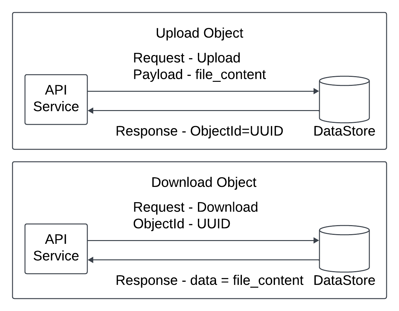
The data store - 3 main components - Data routing service, Placement service, Data Node.
Data Routing Service.
The data routing service provides the restful or grpc APIs to access the data node cluster. It is a stateless servcie that can scale by adding more servers.
It is used to query the placement service to get the best data node to store data.
To read data from data node and return it to the API service.
Placement Service.
It determines which data ndoe (primary or the replicas) should be chosen to store an object. It maintains a virtual cluster map to provide the physical topology of the cluster. The virtual cluster map contains location information for each data node which the placement servcie uses to make sure the replicas are physically separated. The separation is key to high durability.
It monitors all data node through heartbeat. Any node does not send in 15 secs then it is mark asdown in the virtual cluster map.
It is a critical service so we can build a cluster of 5 or 7 placement service nodes with Paxos or Raft consensus protocol. The consensus protocol ensures that as long as mpre than half of the node are healthy the service continues to work.
Example - Placement service cluster 7 nodes, it can tolerate a 3 ndoe failure.
Data Node.
The data node stores the actual object data. It ensures reliability and durability by replicating data to multiple data nodes called a replication group.
Each data node has a data service daemon running on it. The data servcie daemon continuously sends heartbeat to the placement service. The heartbeat message includes information - How much disk drive HDD or SSD does the data node manage? How much data is stored on each drive?
The placement service receives the heartbeat for the first time it assigns an ID for the data node adds it to the virtual cluster map and return the information - a ID of the data node, the virtual cluster map and the place to replicate data.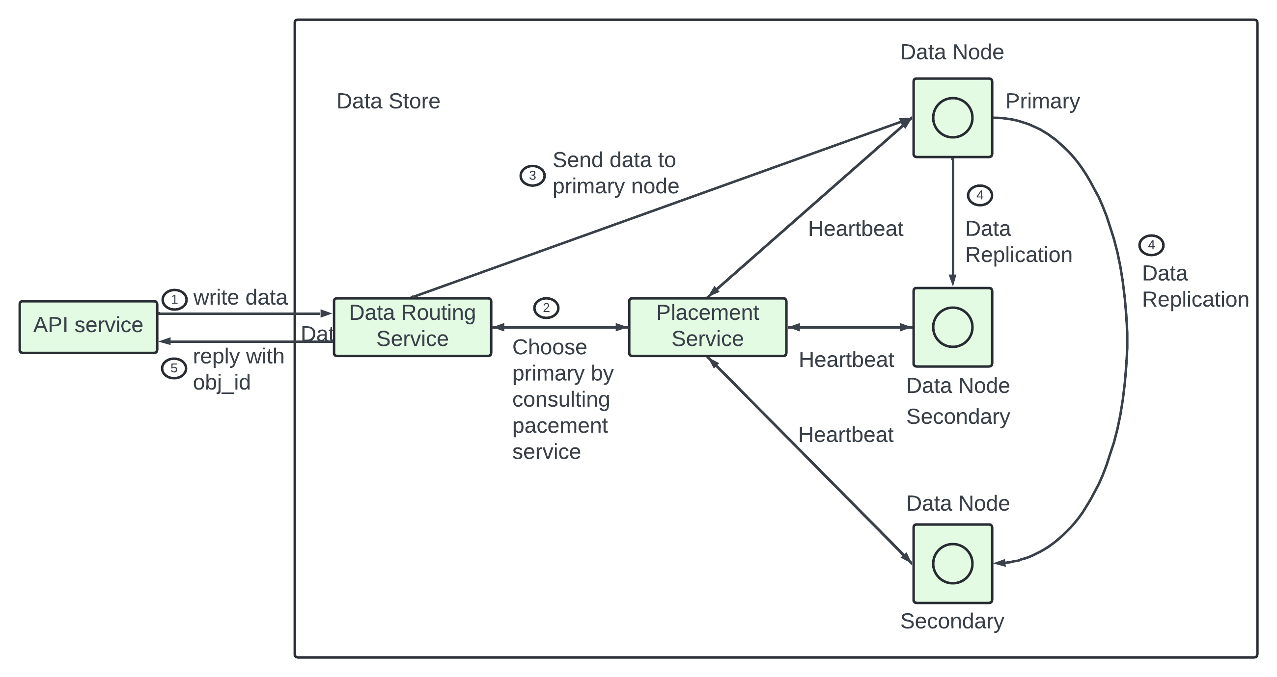
How data persisted in data node?
The API srevcie forwards the object data to the data store.
The API routing service generates a UUID for this object and queries the placement service for the data node to store this object. The placement service see the virtual cluster map and returns the primary data node.
The data routing service sends data to the primary data node with its UUID. The prmary data node saves the data locally and replicates it to two secondary data nodes. The primary respond to the data routing service when data is replicated to all secondary node.
The UUID of the object ObjId is returned to the API service.
In step 2 the UUID is the input and the placement service returns the replication group for the object. How does the placement service do it?
The look up needs to be deterministic and it must survive the addition or removal of replication group. Consistent hashing is a common implementation of such a lookup function.
In step 4 the primary data ndoe replicates data to all secondary ndoes before it returns a response. It makes the data strongly consistent among all data nodes. The consistency comes with latency cost as we have to wait until the slowest replica finishes.
Data is considered as succesfully saved after all 3 nodes store the data - Best consistency and highest latency.
Data is considered as successfully saved after the primary and one of the secondaries store the data - Medium consistency and medium latency.
Data is considered as successfully saved after primary persists the data - Worst consistency and lowest latency.
How data is organized?
A simplesolution store eac object in a stand-alone file. It works but the performance suffers when there are many small files.
The issues when there are many small files.
It wastes many data blocks. A file system stores files in discrete disk blocks. Disk blocks have the same size and the size is fixed when the volume is initiated. The typical block size is 4 Kb and file smaller than 4kb will still consume the entire block.
It could exceed the systems inode capacity. The file system stores the location and other information about a file in a special type of block called inode. In most file system the number of inode is fixed when the disk is initialized. With millions of small files it runs the risk of consuming all inodes. The OS does not handle a large number of inodes even with aggressive caching of file system metadata.
In final storing small objects as file is not good idea.
To address the issue we merge small files into larger files. It works like Write-ahead log WAL. When we save an object, it is appended to an existing read-write file. It reaches the capacity threashold (set to few GBs) the read-write file is markes as read only and th new read-write file is created to get new objects.
When the file is marked as read nly it can only serve read requests.
The write access to the read-write file must be serialized. To maintain the ondisk layout multiple cores processing incoming write requests in parallel must take their turn to write to the read-write file.
In modern server with a large number of core processing many incoming requests in parallel it restricts write throughput. To fix it we can provide dedicated read-write files one for each core processing incoming requests.
Object lookup.
Each data file holding many small objects how does the data node locate an object by UUID?
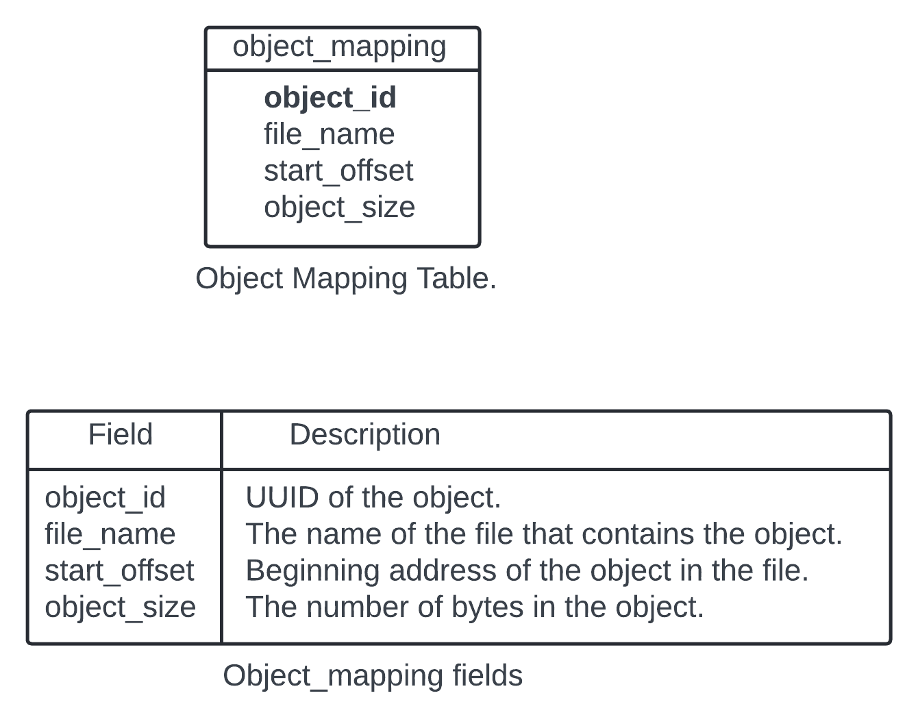
The data node need the information - The data file that contains the object, The starting offset of the object in the data file and the size of the object.
The data schema to support the lookup.
How to deploythe relational database?
The data volume for the mapping table is massive. Deploying a single large cluster to support all data nodes could work but it is difficult to manage. The mapping data is isolated within each data node. There is no need to share it across data nodes. To take advantage of it we could simple deploy a simple relational db on each data node. SQLite is a good option and it is a file based relational database.
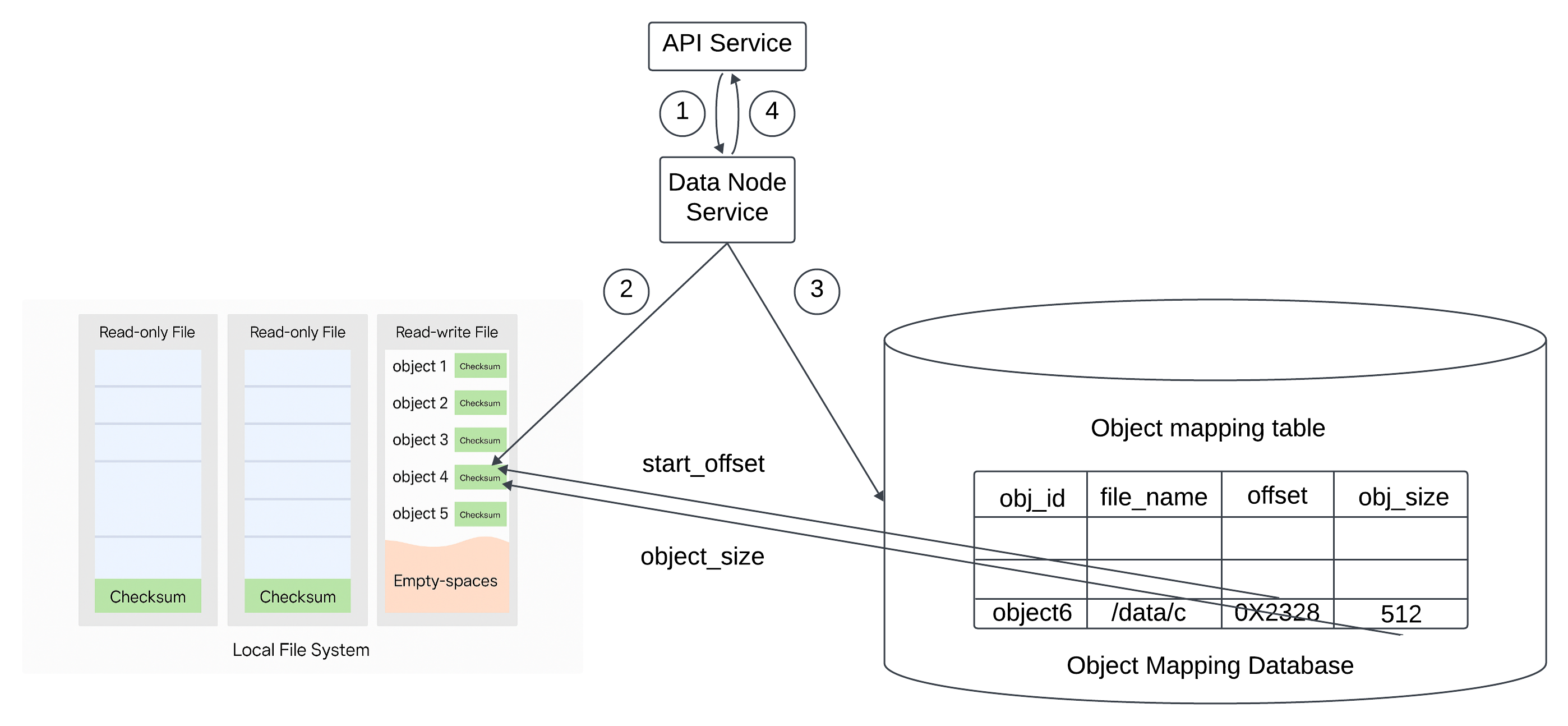
Updated data persistence flow.
How to save a new object in the data node.
The API service sends a request to save a new object names object4. The data node service appends the object named object 4 at the end of teh read-write fiel names /data/c. The new record of object 4 is inserted into the object_mapping table. The data ndoe service returns the UUID to the API service.
Durability.
Data reliability is imp for data storage system.
How to create a storage system that offers 6 nines of durability?
Each failure case needs to be considered and data needs to be properly replicated.
Hardware failure and failure domain.
Hard drive failure are inevitable no matter which media we use. Some storage media may have better durability than others but we cannot rely on a single hard drive to achieve out durability objective.
A proven way to increase durability is to replicate data to multiple hard drives so a single disk failure does not impact the data availability.
In our design we replicate data 3 times. The spinning hard drive has an annual failure rate of 0.81% This number depends on the model and make. Making 3 copies of dta given us 1-0.0081^3 = ~0.999999 reliability.
To get complete durability evaluation we need to consider the impacts of differerent failure domain. A failure domain is a physical or logical section of the environment that is negatively affected when a critical sevice experiences problem. In a modern data center a server is put into a rack and the racks are grouped into row/floors/rooms. Each rack shares the network switches and power all the servers in a rack are in a rack level failure domain.
A modern server shares components like the mother board, processor, power supply, HDD drives. The component in a server are in a node level failure domain.
Example of a large scale failure domain isolation. Data centers divide infrastructure that shares nothing into different Availability zones, We can replicate the data to different Availability zones to minimize the failure impact.
Image MultiDataCenterReplication present.
Erasure Coding.
Making 3 full copies of data gives roughly 6 nines of data durability.
Any other option to increase durability?
Erasure coding one option. It chunks the data into smaller pieces(placed on different servers) and creates parities for redundancy. In the event of failure we can use chunk data and parities to reconstruct the data. Example (4+2 erasure coding).
ErasureCoding Image present.
Data broken into 4 even sized data chunks d1 to d4. teh formula is usedto calculate th eparities p1 and p2. To give an example p1 = d1+2d2-d3+4d4 and p2 = -d1+5d2+d3-3d4. Data d3 and d4 are lost due to node crashes. The formula is used to reconstruct lost data d3 and d4 using the known value of d1,d2, p1 and p2.
How it work in failure domain?
Example 8+4 erasure coding set up breaks the data into 8 chunks and calculates 4 parities. All pieces of data have the same size.
All 12 chunks of data are distributed across 12 different failure domains. The mathematics behind the erasure coding ensures that the original data can be reconstructed when at most 4 nodes are down.
Compared to replication where the data router only needs to read data for an object from one healthy node in erasure coding the data router has to read data from at least 8 healthy ndoes. It is an architectural design tradeoff. It is a complex solution with a slower access speed in exchange of high durability and lower storage cost. In object storage where the main cost os storage the tradeoff might be worth it.
How much extra space does erasure coding need?
Every two chunks of data we need one oarity block so the storage overhead is 50%. While in 3 copy replication the storage overhead is 200%.
Image ExtraSpaceForReplicationAndErasureCoding present.
ExtraSpaceforRelicationAndErasureCoding.
In general erasure coding get 11 nines durability.
| Component | Replication | ErasureCoding |
|---|---|---|
| Durability | 6 nines of durability (data copied 3 times) | 11 nines of durability(8+4 erasure coding). It wins. |
| Storage Efficiency | 200% storage overhead. | 50% storage overhead. It wins. |
| Compute Resource | No computation. It wins. | Higher usage of computation resources to calculate parities. |
| Write performance. | Replicating data to multiple nodes. No calculation is needed. It wins. | Incraesed write latency as we need to calculate parities before data is written to disk. |
| Read performance | In normal operations reads are served from the same replica. Reads under a failure mode are not impacted as reads can be served from a non-fault replica. It wins. | In normal operation, every read has to come from multiple nodes in the cluster. Reads under a failure mode are slower as the missing data must be reconstructed first. |
Repliction in latency sensitive application and erasure coding in minimize storage cost.
Correctness Verification.
Erasure cosing increases data durability at comparable storage costs. Now handing data corruption.
If a disk fails completely and the failure can be detected it can be treated as data node failure. In this case reconstruct data using erasure cosing. Inn-memory data corruption is a regular occurrence in large scale system.
It can be addressed by verifying checksums between process boundaries. A checksum is a small sized block of data that is used to detect data errors.
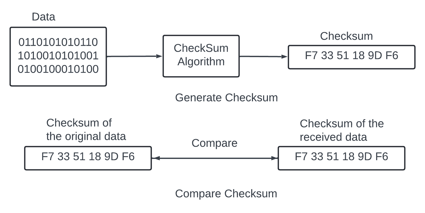
There are many checksum algorithm like MD5, SHA1, HMAC.
A good checksum algorithm outputs a different value for a small change made to the input. In out design checksum MD5 append the checksum at the end of each object. Before the file is marked read-only we add checksum of the entire file at the end.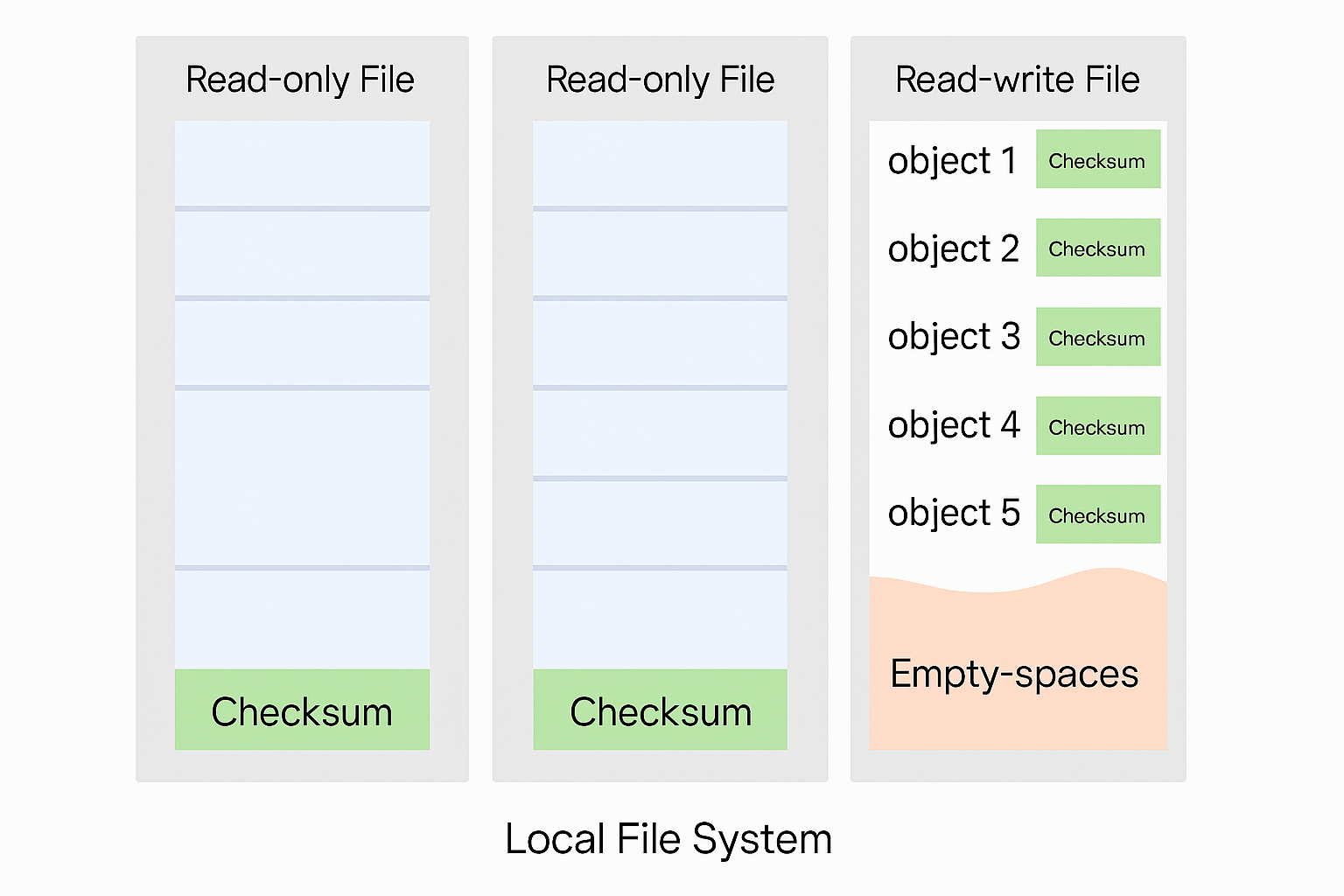
Repeat the steps until 8 pieces of data are returned. Then reconstruct the data and send it back to the client.
Metadata data model.
The database schema and then dive into scaling the database - Schema needs to support the 3 queries - Query 1 - Find objectID by the object name. Query2 - Insert and delete an object based on the object name. Query3 - List objects in a bucket sharing the same prefix.
We need two database table bucket and object.
Scale the bucket table.
There is a limit on the number of buckets a user can create teh size of teh bucket table is small. 1 million customers and ecah own 10 nucket and each record takes 1KB. It mesna 10GB of storage space (1 million * 10 * 1KB). The entore table can fits in modern database server. A single db server might not have enough CPU or network bandwidth to handle all read requests. We can spread the read load among multiple database replicas.
Scale the object table.
The object table holds the object metadata. The dataset at our design scale will not fits in a single database instance. We can scale the ovbject table by sharding.
One option shard by the bucket_id so all teh object under the same bucket are stored in one shard. It does not works as it causes hotspot shards as the bucket might contains billions of obects.
Another option shard by the object_id. It evenly distributes the load. In this case we will not be able to perform query 1 and 2 efficiently as those queries are based on the URI.
We are choosingto shard by the combination of bucket_name and object_name. The choice is correct as most of the metadata operations are based on the object URI example finding the object ID by the URI or uploading an object via URI. To evenly distribute the data we can use the hash of the <bucket_name, object_name> as the shading key.
The sharding scheme it is easy to suport first two queries but the last one is less obvious.
Listing objects in a bucket.
The object store arranges files ina flat structure instead of a heirarchy like in a file system.
An object can be accessed using a path in this format s3://bucket-name/object-name Example s3://mybucket/abc/d/e/f/file.txt contains - Bucket name mybucket, object nema abc/d/e/f/file.txt
To help user organize the objects in a bucket S3 introduces a concept called ‘prefixes’. A prefix is a string at the beginning of the object name. S3 uses prefixes to organie the data in a way similar to directories. Prefixes are not directories.
Listing a bucket by prefix limits the results to only those objects names that begin with the prefix.
In the example with the path s3://mybucket/abc/d/e/f/file.txt the prefix is abc/d/e/f/ . The AWS S3 listing command has 3 typical uses.
List all bucket owned by auser. The command aws s2 list-buckets.
List all objects in a bucket that are at the smae level as the specified prefix. Teh command - aws s3 ls s3://mybucket/abc/ In this mode, the objects with more slashes in the name after the prefix are rolled up into a common prefix. Example with these objects in the bucket.
CA/cities/losangeles.txt
CA/cities/sanfrancisco.txt
NY/cities/ny.txt
federal.txt
Listing the bucket with the ‘/’ prefix would return these results with everything under CA/ and NY/ rolled up into them.
CA/
NY/
federal.txt
Recursively list all objects in a bucket that shares the same prefix. Teh command looks like aws s3 ls s3://mybucket/abc/ --recursive Using the same example lising the bucket with the CA. prefix would return these results.
CA/cities/losangeles.txt
CA/cities/sanfrancisco.txt
Single Database.
Listing command with a single database. List all buckets owned by a user SELECT * FROM bucket WHERE owner_id={id} To list all object in a bucket that share teh same prefix SELECT * FROM object WHERE bucket_id="123" AND object_name LIKE abc/%``
Any object with more slashes in their names after the specifies prefix are roleld up in the application code.
Teh same query supports the recursive listing mode. The application code list every object sharing the same prefix without performing any rollups.
Distributed database.
When the metadata table is sharded it is difficult to implement the lsiting fucntion as we dont know which shards contains the data.
Easy solution - Run a search query on all shards and then aggregate the results. To get this, The meta data servcie queries every shards by running the query SELECT * FROM object WHERE bucket_id="123" AND object_name LIKE 'a/b/%' the metadata service aggregates all objects returned from each shards and return the result to the caller.
This solution works but implementing pagination is complicated.
How pagination works in a simple case with a single database.
Return list of 10 objects for each page the SELECT query would start wih SELECT * FROM object WHERE bucket_id="123" AND object_name LIKE 'a/b/%' ORDER BY object_name OFFSET 0 LIMIT 10
The OFFSET and LIMIT restricts te result to the first 10 objects. In the next call the user sends the requests with a hint to the server so it is known to construct the query for te second page with an OFFSET of 10. The hint is usually done with a cursor that teh server returns with each page to the client.
The offset information is encoded in the cluster. The client can include the cursor in the request for the next page. Reservoir decodes the cursor and uses the offset information to construct the query for the next page. the query for the second page will be SELECT * FROM object WHERE bucket_id="123" AND object_name LIKE 'a/b/%' ORDER BY object_name OFFSET 10 LIMIT 10
The client-server requets loop continues until the server returns a special cursor that marks the end of the entire listing.
The pagination is complicated for sharded database. The objects are distributed across shards and the shards would likely return a varying number of results Some would return a full page of 10 objects while the other will be partial. The application code will receive results from every short aggregate and sort them and then return only the page of 10. The object that did not include it in this round must be considered again for the next round. This means each shard would likely have a different offset. The server track the offset for all the shards and associate those offset with the cursor. If there are 100 of shards there will be hundreds of offsets to track.
Solution - Object storage is tuned for vast scale and high durability and object listing performance is not a priority. All commercial object storage support object listing with sub optimal performance. To take advantage of this we can denormalize the listing data into a separate table sharded by bucketId. This table is only used for listing object. With this setup even buckets with billions of objects would offer acceptable performance it isolates the listing query to a single database which greatly simplifies the implementation.
Object versioning.
It is a feature that keeps multiple versions of an object in a bucket We can restore object that are deleted or overwritten.. Example we can modify a document and save it under the same name inside the same bucket.
Without versioning the old version of the document is replaced by the new version in the metadata store. The old version of the document is marked deleted so its storage space will be reclaimed by the garbage collector.
With versioning the object storage keeps all previous version of the document in the metadata store and the old version will never mark as deleted in the object store.
First we need to enable versioning on the bucket.
Client sends an HTTP PUT request to upload an object script.txt. The API service verifies if the user has the right permission on the bucket once verified it uploads the data to the data store. the data store purses the data as a new object in return and uuid to the api service. The API service calls the metadata store to store the metadata information of the object.
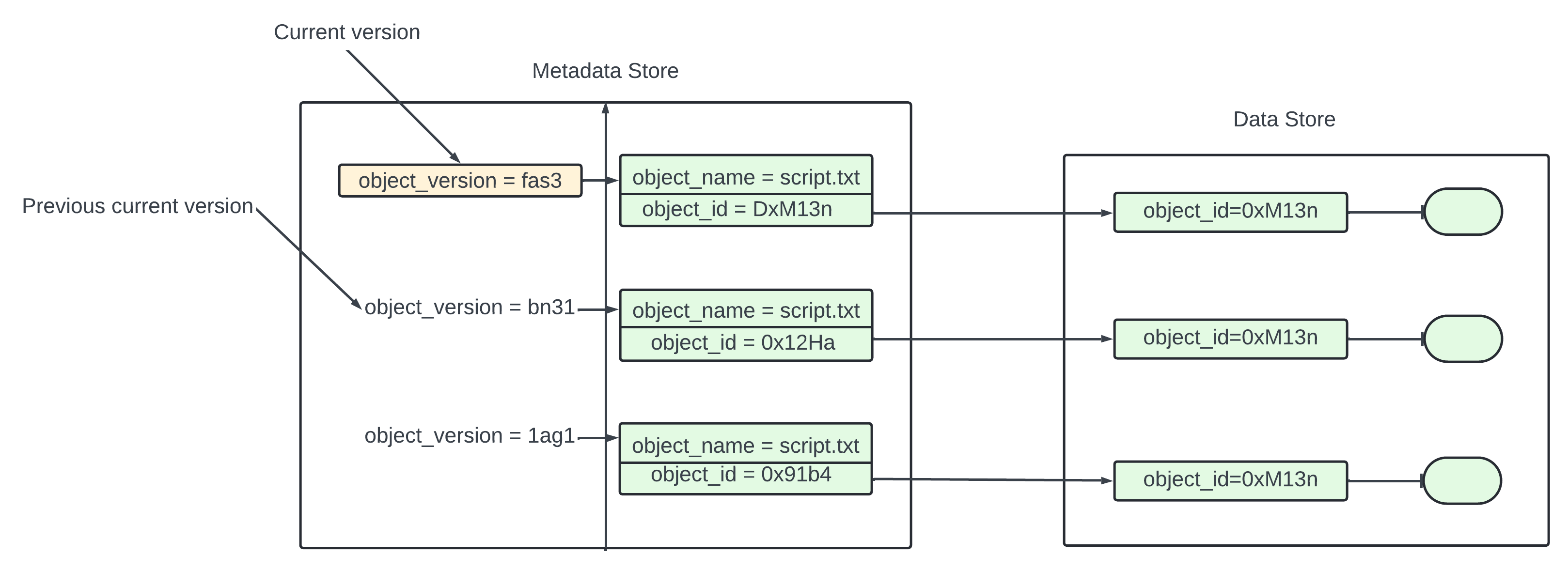
To support versioning the object table for the metadata store has a column called object_version that is only used if versioning is enabled. Instead of overwriting the existing record and new record is inserted with the same bucket_id and object_name as the old record but with a new object_id and object_version. The object_version is a TIMEUUID generated when the new row is inserted.
Any database we sleect it is efficinet to look up the current version fo an object. The current version has the largest TIMEUUID of all the entries with the same object_name.
When we delete an object all versions remain in the bucket and we insert a delete market.
Image DeleteObjectByInsertingDeleteMarker Image present.
Delete object by inserting a delete marker.
A delete marker is a new version of the object and it becomes the current version of the object once inserted. Performing GEt requets when the current version of the object is a delete marker returns a 404 object not found error.
Optimizing upload of large files.
In the estimation there got that 20% of the object are large. Uploading the large file directly will take long time. Any network connection fails in the middle then we have to start over. A better solution to slice the large data into small parts and upload them individually. All parts are uploaded store reassemble the object from the parts. The process is called multipart upload.
Image MultiPartUpload present.
MultipartUpload.
Client calls the objectstorage to initiate a multipart upload. The data store returns an uploadID The client splits the large file into small objects and starts uploading. The size of the file is 1.6GB and the clients plits into 8 parts si each part 200MB in size. The client uploads the first parts to the data store with the upladID it received in step 2.
When a part is uploaded the data store returns a ETAg and it is the md5 checksum of that part. It is used to verify multipart uploads.
After all parts are uploaded the clients sends a complete multipart upload request which include the uploadID, part number and ETag.
The data store reassemble the object based on teh part number. Object is very large and it may take some time. After the reassemble complete it returns a success message to the client.
One potential problem the old part are no longer useful after the object has been reassembled from them. To solve the issue we can use garbage collection service to free up space from parts that are no longer needed.
Garbage Collection.
It is the process of reclaiming storage space no longer in use. There are a few ways data might become garbage - Lazy object deletion An object marked deleted at delete time without actually being deleted. Orphan data Half uploaded data or abandoned multipart upload. Corrupted data data that failed the checksum verification.
The garbage collector does not remove objects from the data store directly. Deleted objects will be periodically cleaned up with a compaction mechanism. It also reclaims unused space in replicas. For replication we delete the object from both primary and backup node. For eraure coding if we use(8+4) setup we delete the object from all 12 nodes.
How compaction works?
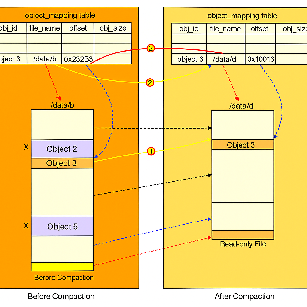
The garbage collector copies object from /data/b to the new file names data/d. The garbage collector skips Object2 and 5 as the delete flag is set to true for both of them.
All objects are copied the garbage collector updates the object_mapping table. Example the obj_id and obj_size fields of Object 3 remains the same but the file_name and start_offset are updated to reflect its new location. To ensure data consistency it is good to wrap the update operations to file_name and start_offset in the db transaction.
The size of the new file smaller than the old file. To avoid creating number of small files the garbage collector waits till there are large number of read only files to compact and the compaction process appends objects from many read-only files into a few large new files.
286 missing.