Design Metric Monitoring and Alerting System.
Building the system for the internal system like in-house system or SaaS service like Splunk or Datadog - Internal use only.
What metric to collect - Operational system metric. It can be low level usage data of the operating system like CPU load, memory usage, disk space. It can be high level such as request per second or the service or the running server count of a web pool.
Scale of the infrastructure - 100 million daily active users, 1000 server pools and 100 machine per pool.
How long to keep the data - 1 year retention.
Reduce the resolution of the metric data for long-term storage - New data for 7 days. After 7 days, you can roll them up to 1 minute resolution for 30 days and after 30 days you can further roll them up at a 1 hour resolution.
Supported alert channel - Email, Phone, PagerDuty. Webhooks.
Need to collect logs like error logs or access log - No.
Need o support distributed system tracing - No.
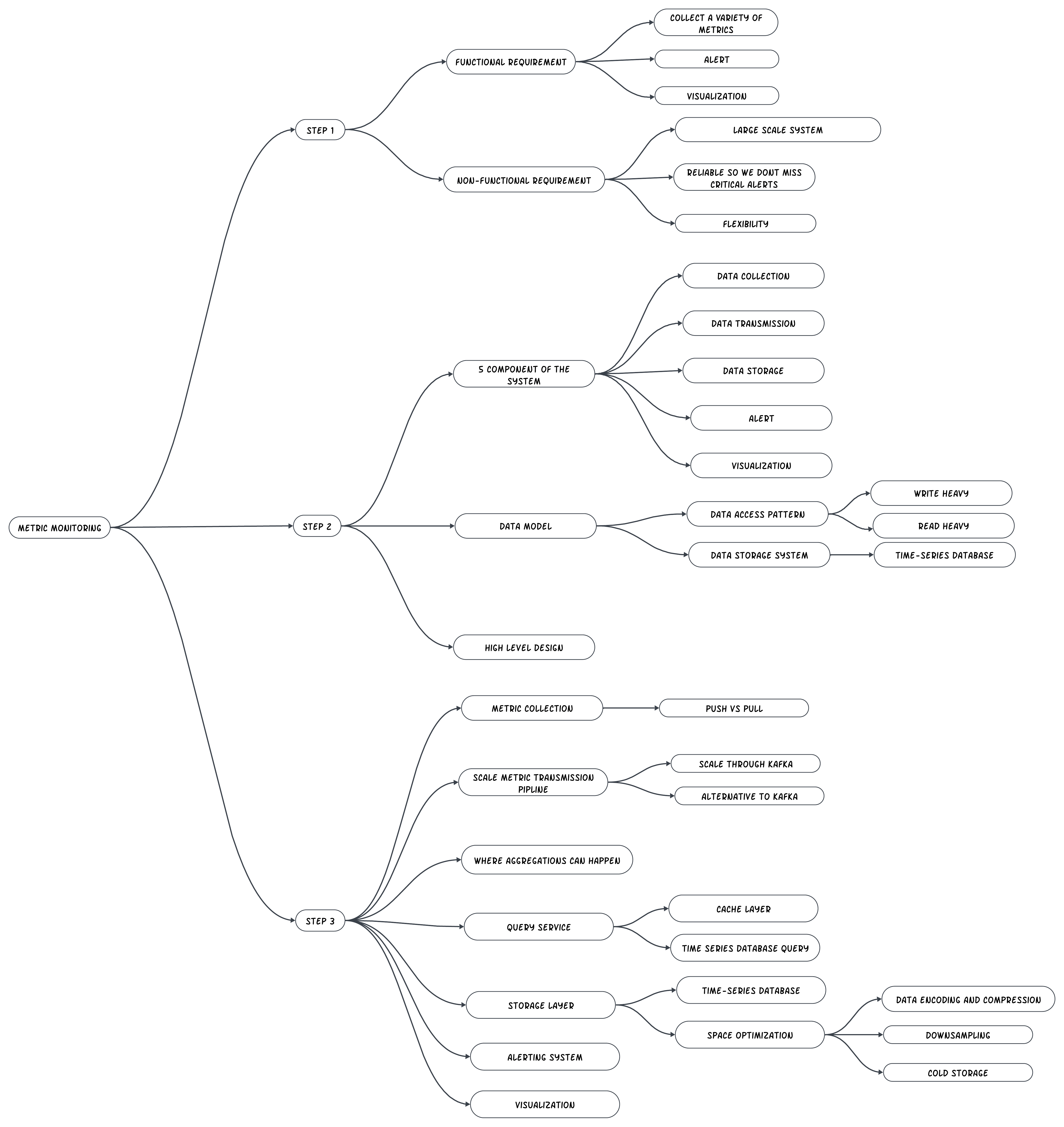
High level requirements and assumptions.
Functional Requirements.
Infrastructure monitored is large scale - 100 million DAU. Assume 1000 server pools, 100 machines per pool, 100 metrics per machine = 10 million metrics.
1 year data retention.
Data retention policy - raw form for 7 days, 1 minute resolution for 30 days, 1 hour resolution for 1 year.
Metric monitored - CPU usage, Request count, Memory usage, Message count in message queues.
Non-Functional Requirements.
Scalability - The system should be scalable to growing metrics and alert volume.
Low latency - The system needs to have low query latency for dashboard and alerts.
Reliability - The system should e highly reliable to avoid missing critical alerts.
Flexibility - Pipeline should be flexible enough to integrate new technology in future.
Requirements Out of scope.
Log Monitoring - The Elasticsearch Logstash Kibana ELK stack is very popular for collecting and monitoring logs.
Distributed System tracing - Distributed tracing refers to a tracing solution that tracks service requests as they flow through distributed systems. It collects data as requests go one service to another.
High level design.
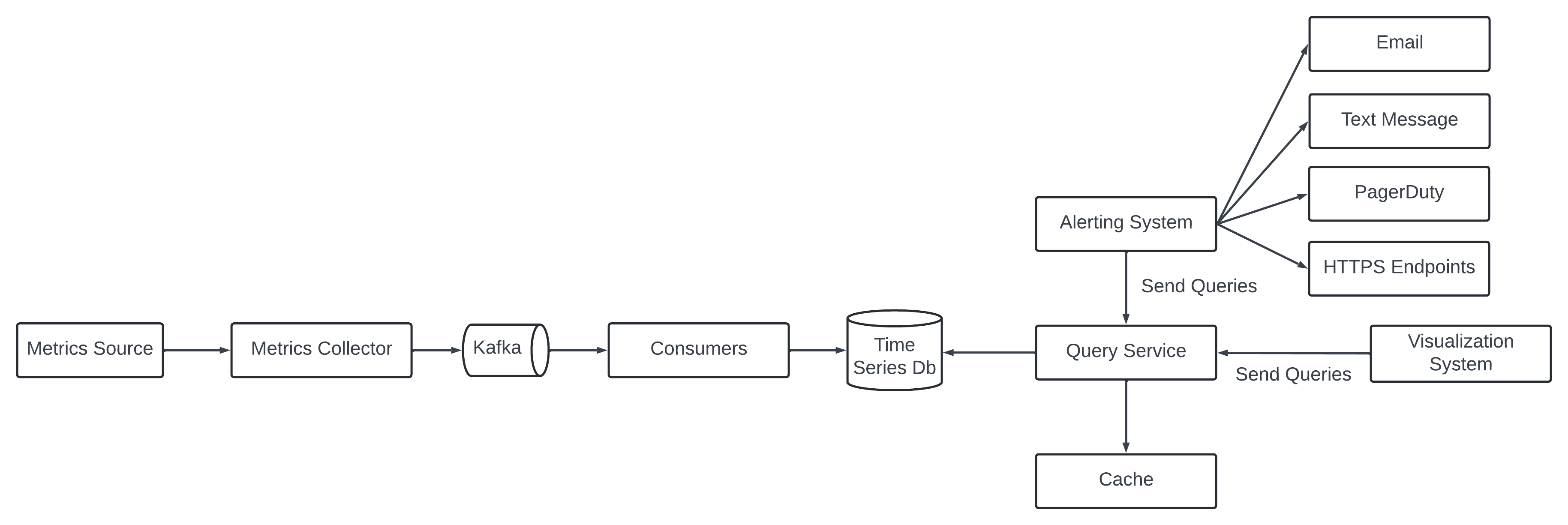
Metric monitoring and alerting system have 5 main components.
Data Collection - Collect metric data from different source.
Data transmission - Transfer data from sources to the metrics monitoring system.
Data Storage - Organize and store incoming data.
Alerting - Analyze incoming data, detect anomaly and generate alerts to communication channels.
Visualization - Present in graph, charts.
Data Model.
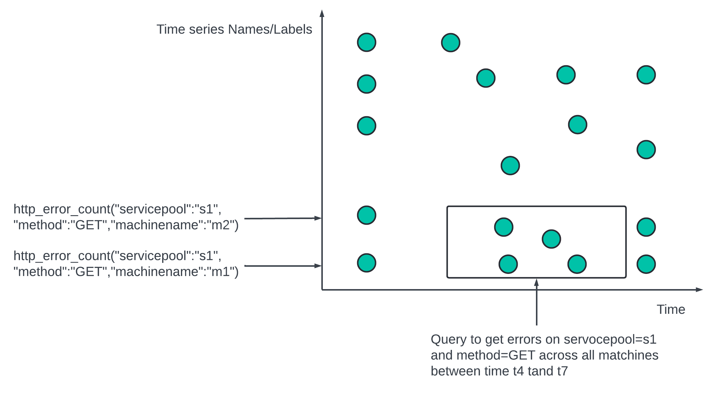
Metric data is recorded in time series. The series can be identified by its name and set of labels
What is the CPU load on production server instance i631 at 20:00?
Data visible in chart and can be placed in a table.
metric_name - cpu.load
lavels - host:i631,env:prod
timestamp - 1613707265
value - 0.29
In the example the timeseries is represented by the metric name, the labels and the single value at the specific time.
What is the average CPU load across all web servers in teh us-west region for the last 10 min?
We can pull up the data from the storage where the metric name is CPU.load and the region label is us-west.
CPU.load host=webserver01,region=us-west, 1613707265 50
CPU.load host=webserver02,region=us-west, 1613707265 89
CPU.load host=webserver01,region=us-west, 1613707265 98
CPU.load host=webserver01,region=us-west, 1613707265 89
CPU.load host=webserver01,region=us-west, 1613707265 50
Average CPU load can be computed by averaging the values at the end of the line. The format of the line in the example is called Line Protocol.
Each time series consists of metric name, set of tags or labels and an array of values and timestamps.
Data Access pattern.
The write load is heavy. There are many time-series data points at any moment. There are 10 Million metrics per day.
The read load is spiky. The visualization and alerting services send queries to the database - depending on the access patterns of the graphs and alerts the read volume can be heavy.
The system is write load heavy and read load spiky.
Data Storage System.
No recommended to use own storage or use general purpose storage system like SQL.
SQL is good to support time-series data but at this scale need expert level skill. It is not optimized for operations against time-series data. Example - Computing moving average in rolling time window need complicated SQL difficult to reading. To support the tagging or labeling we need to add an index for each tag and relational database is not good under constant heavy write load.
NoSql - Cassandra BigTable can be used for time series database. It need deep knowledge of the internal workings to make a scalable schema for storing and querying time series data.
Time-series database optimized to handle high volume - OpenTSDb, MetricsDb.
OpenTSDb - distributed time-series database based on Hadoop and HBase - running on Hadoop/HBase cluster add complexity.
Twitter uses MetricsDb. Amazon uses Timestream.
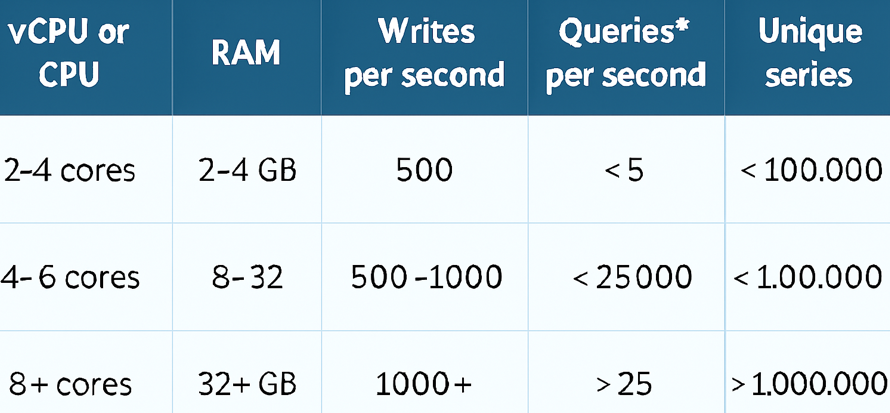
According to Db-engines most popular time series db are InfluxDB and Prometheus - designed to store large volume of data - It rely on in-memory cache and on-disk storage.
InfluxDb 8 core and 32 GB RAM can handle 250K write per second.
TimeSeries DB in-depth not needed - Metric data is time-series and InfluxDb as storage used.
Time-series db is efficient in aggregation and analysis of amount of time-series data by labels called tags in some db. InfluxDb builds indexes on labels to do the fast lookup of time-series by labels. The main point to make sure that each label is of low cardinality(having a small set of possible values).
High-Level Design.
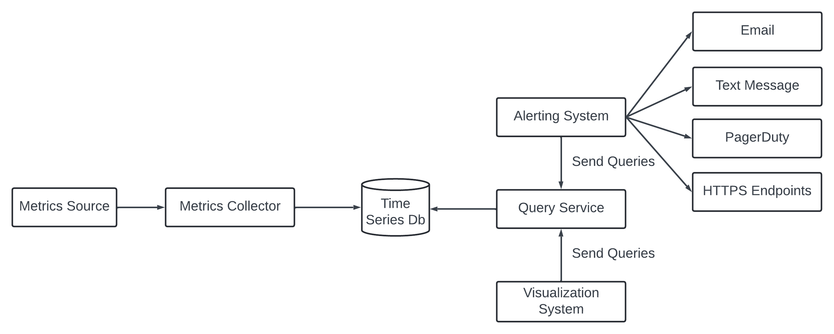
Metric Source - It can be application server, SQL databases, message queues.
Metrics Collector - It gathers metrics data and writes data into the time-series db.
Time-series - Store metric data in time-stamp. It provide custom query interface for summarizing a large amount of data - index on labels to facilitate the fast lookup of the data by labels.
Query service - It ease the query and retrieve data from the database. It can be a thin wrapper on the database. It can be replaced by the time-series database own query interface.
Design Deep Dive.
Imp components - Metric collection, Scaling the metric transmission pipeline, Query service, Storage layer, Alerting System, Visualization System.
Metric Collection.
In the high level design the metric source and the metric collector are the part of this section. Metric collection like counters or CPU usage - data loss is not an issue.
Pull vs Push Models.
There are 2 ways metrics data can be collected - push or pull.
Pull Model.
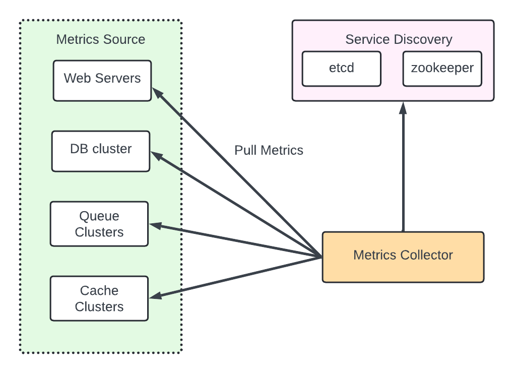
The metric collector need to know the complete list of service end points to pull data. Naive approach - Use a file to hold DNS/IP information for every endpoint on the “metric collector” servers. Issue in large scale system where server added and removed frequently. Need to ensure it does not miss out any metric from any new server.
Using reliable, maintainable and scalable Service Discovery provided by etcd, zookeeper wherein services register the availability and the metrics collector can be notified by the Service Discovery component when the endpoint changes.
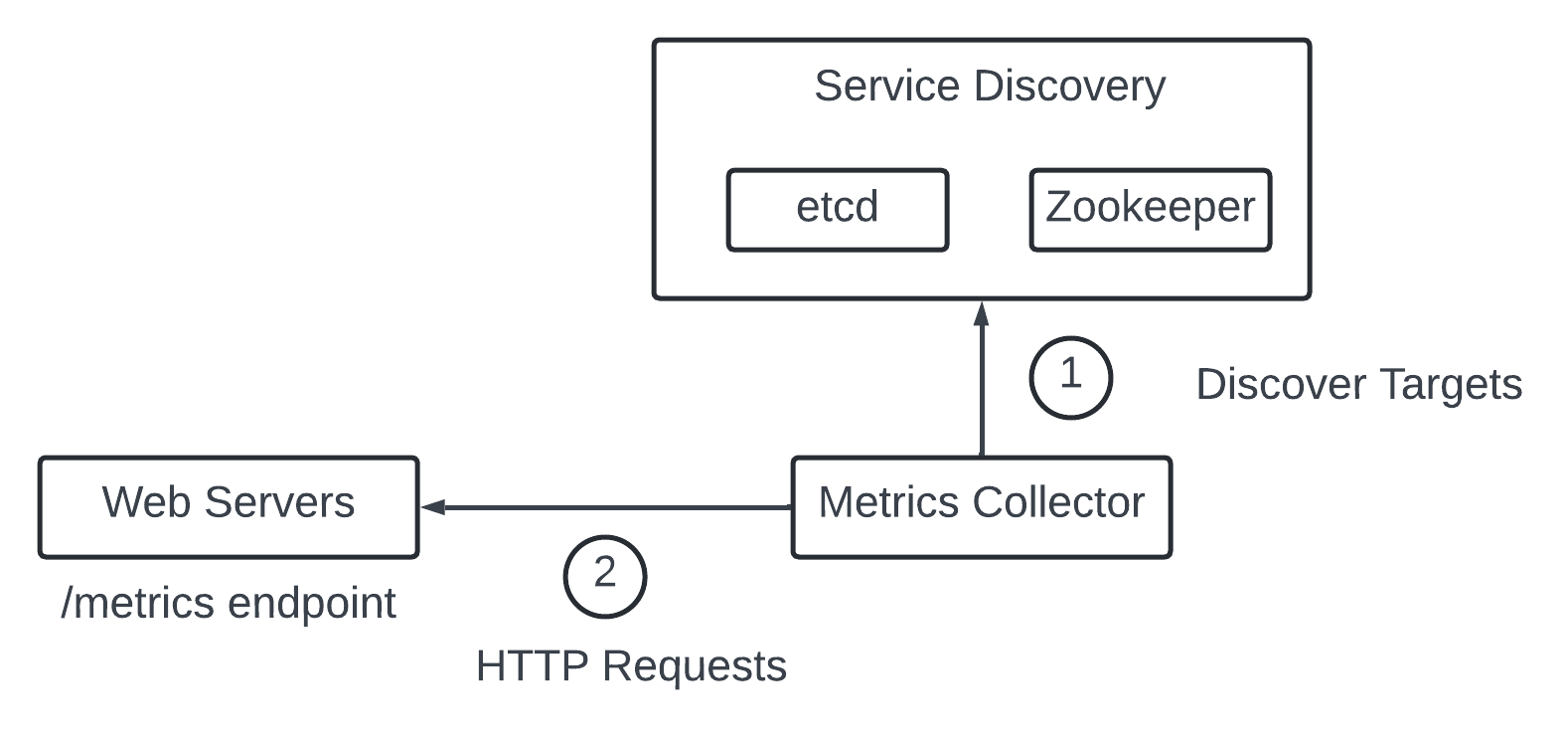
1 - The metric collector fetches configuration metadata (pilling interval, Ip address, timeout and retry parameters) of service endpoints from Service Discovery.
2 - The metric collector pulls data vis HTTP endpoint - to expose the endpoint a client library need to be added to the service.
3 - The metric collector register a change event notification with Service Discovery to receive an update when endpoint change. Alternately, the metrics collector can poll for endpoint change periodically.
At our scale we need pool of metric collector to handle all the servers. Issue in multiple collector - multiple instances try to pull data from the same resource and produce duplicate data. There should be a coordination schema to avoid the issue.
One approach - designate each collector to a range in a consistent hash ring and then map every dingle server being monitored by its unique name in the hash ring - one metric source server is handled by one collector.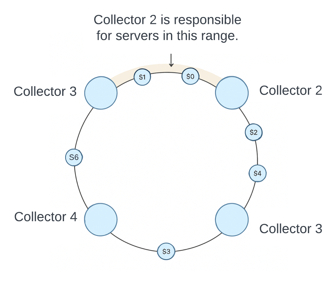
There are 4 collectors and 6 metrics source servers. Each collector is collecting metric from distinct set of servers. C2 is collecting metric from S1 and S0.
Push Model.
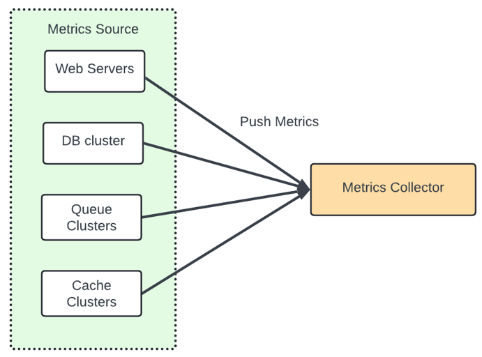
A collection agent is installed on every server being monitored.
Collection Agent - A piece of long running software that collects metrics from the services running on the server and pushes the metric periodically to the metrics collector. It will aggregate metric like counter locally and then send to the metric collector.
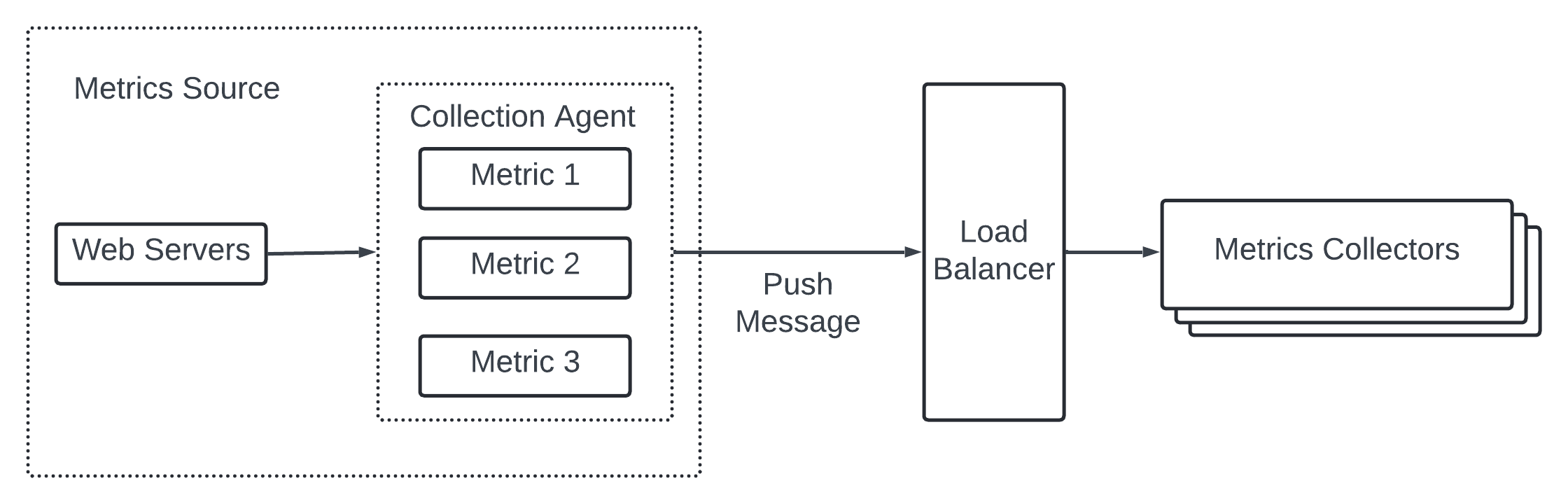
Aggregation reduce the volume of data sent to the metric collector. The push traffic is high and metric collector rejects the push with an error - the agent could keep a small buffer of data locally in disk and resend them when traffic is low.
On the other hand of the servers are in an auto-scaling group where they are rotated out frequently then holding data locally temporarily result in data loss when the metric collector falls behind.
To prevent the metric collector from falling behind in push model - the metric collector should be in auto-scaling with a load balancer in front of it. The cluster should scale up and down based on CPU load of the metric collector servers.
Push or Pull?
Both are good and used in production system
Example of pull architecture - Prometheus. Example of Push architecture - Amazon CloudWatch, Graphite.
Know the adv and dis-advantage is good to discuss in interview rather than picking.
| Advantage of Pull | Advantage of Push. |
|---|---|
| It is an easy debugging. The /metrics endpoint on server used for pulling metrics can be used to view metric anytime. Pull wins. | Some of the batch jobs might be short-lived and does not exists long enough to be pulled. Push wins. It can be configured by a push gateway for the pull model. |
| No response in pull - the application server might be down. Easy to work in the hand of developer. Pull wins. | Metric collector does not receive any record - it can be network issue. |
| Servers pulling metric requires all endpoint to be reachable, It need more network infrastructure. | Metric collector set up with a load balancer and an auto-scaling group - get the data from anywhere and nos etup needed. Push wins. |
| Uses TCP. | Uses UDP. Push model provide low latency transport of metrics. Counter argument - The effort of establishing a TCP connection is small compared to sending the metric payload. |
| Data authenticity - Application server to collect metric are defined in config files. Metrics gatheres are guaranteed to be authentic. | Any kind of client can push metric to the metrics collector. It can be fixed by whitelisting servers from which to accept metrics or by requiring authentication. |
Scale the metrics transmission pipeline.
Transmission pipeline include metric collector and the time series db in the high level design.
Metric collector is a cluster of servers and the cluster receives huge amount of data. It is set up for autoscaling to ensure there are adequate number of collector instances to handle the demand.
There is risk of data loss when the time series database is unavailable. To mitigate the problem - Introduce a queue component.
The metric collector send metrics data to the queuing system like Kafka - the consumer or streaming processing service push the data to the time-series database.
Advantage - Kafka used as highly reliable and scalable distributed messaging platform. It decouple the data collection and data processing services from each other. It prevent data loss using the retention policy.
Scale through Kafka.
There are steps to scale the system.
Configure the number of partitions based on throughput requirements. Partition metrics data by metrics names so that consumer can aggregate data by metrics name.
Further partition metrics data with tags and labels.
Categorize and prioritize metrics so that important metrics can be processed first.
Alternate to Kafka.
Maintaining a kafka production scale is big deal. There are large scale monitoring ingestion systems in use without using queue.
Facebook’s Gorilla in memory time series db is an example designed to maintain highly available for write - in partial network failure.
Where aggregation can happen.
Metrics aggregated in different places - in collection agent (client side), ingestion pipeline(before writing to storage), query side(after writing to storage).
Collection agent - Simple aggregation logic - Aggregate a counter every minute before it is sent to the metrics collector.
Ingestion Pipeline - Aggregate data before writing to the storage - stream processing engines like Flink. The write volume is low only calculated result is written to the database. Handling late arrival of data is challenging and loss of data precision and flexibility as not storing the raw data.
Query side - Raw data is aggregated over a time period at query time. There is no data loss - the query speed might be slower as the query result is computed at query time and is run against the entire dataset.
Query Service.
The query service comprises a cluster of query servers - which access the time-series databases and handle requests from the visualization or alerting systems.
A dedicated set of query servers decouples tie-series databases from the clients(visualization and alerting). It give flexibility to change the time-series database or the visualization and alerting system.
Cache Layer.
To reduce the load in the time-series database and make query service more performant - cache server are added to store query results.
There is no imp need to add own abstraction (query service) as most industrial scale client system have powerful plugins to interface with time-series database. A popular time series database there is no need to add own caching.
Time-series database query language.
Most popular monitoring system like Prometheus and InfluxDb don’t use SQL - own query language. It is difficult to code in SQL.
Code to compute exponential moving average in SQL.
SELECT id, temp,
	   avg(temp) OVER (PARTITION BY group_nr ORDER BY time_read)
	   AS rolling_avg
FROM (
	SELECT id, temp, time_read, interval_group,
		id - row_number() OVER (PARTITION BY interval_group ORDER BY time_read)
		AS group_nr
	FROM (
		SELECT id, time_read,
			"epoch"::timestamp + "900 seconds"::interval * (
			extract(epoch FROM time_read)::int4/900) AS interval_group,
			temp FROM readings
	) t1
) t2
ORDER BY time_read;
In Flux - language optimized in time series analysis (used in InfluxDb) it is much easier.
FROM(db:"telegraf")
		|> range(start:-1h)
		|> FILTER(FN: (r) => r._MEASUREMNET == "foo")
		|> exponentialMovingAverage(size:-10s)
Storage Layer.
Choose a time-series database carefully.
Research paper by Facebook mention at least 85% of all queries to the operational data store were for data collected in the past 26 hours. Use a time-series database that harness this property - impact in the system performance.
Space Optimization.
The amount of metric data to store is enormous. Strategies to tackle the issue.
Data encoding and compression.
It reduce the size of data significantly. It is usually built in feature in time-series database.
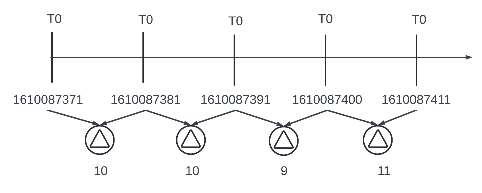
1610087371 and 81 differs by only 10 sec and it takes 4 bits to represent instead of the full timestamp of 32 bits. Rather than storing the absolute value - the delta of the values can be stored along with one base value like 1610087371, 10, 10, 9, 11.
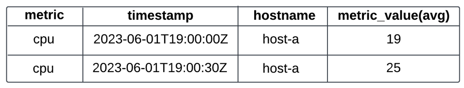
Downsampling.
A process of converting high resolution data to low resolution to reduce overall disk usage. Data retention is 1 year we can downsample old data. Example- Retention 7 days - no sampling, Retention - 30 days, downsample to 1 minute resolution, Retention - 1 year, downsample to 1 hour resolution.
Example - Aggregate 10 second resolution data to 30 second resolution data.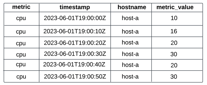
The storage of inactive data that are rarely used. The cost is low and we can use third party solution.
Alerting System.
The alert flow works as follow
1 - Load config file to cache server. Rules are defined as config file on the disk in YAML format. Example of alert rules.
- name: instance_down
rules:

# Alert for any instance that is unreachable for >5 minutes.
- alert: instance_down
	expr: up == 0
	for: 5m
	labels:
	severity: page
2 - The alert manager fetches alert configs from the cache.
3 - Based on the config rules alert manager calls the query service at a predefined interval. If the value violates the threshold the alert event is created. The alert manager is responsible for the following - Filter, merge and dedupe alerts.
Example of merging alerts triggered within one instance within a short amount of time.
Access Control - Restrict access to certain alert management operations to authorized individual.
Retry - The alert manager checks alert states and ensures a notification is sent atleast once.
4 - The alert store is a key-value database like Cassandra that keeps the state(inactive, pending, firing, resolved) of all alerts. It ensures a notification is sent at least once.
5 - Eligible alerts are inserted to Kafka.
6 - Alert consumers pull alert from Kafka.
7 - Alert consumers process alert events from Kafka and send notification over different channels like email, text message, PagerDuty or Http endpoint.
Alerting System - build vs buy.
There are many industrial scale alerting system that provide tight integration with the time-series database. They integrate with any notification channel like email. Good to go with any existing system.
Visualization System.
Visualization is built on top of data layer. Metrics can be shown on metric dashboard and alert in the alert dashboard. Use an off-the-shelf system. Example - Grafana can be a good example. It integrate well with time-series database.