System Design ByteByteGo Videos.
What happens when you type a URL into a browser?
https://youtu.be/AlkDbnbv7dk?si=ng-q1p3bEIXeurCM
Hi, welcome to the first episode of ByteByteGo system design video series. In these videos, we Here in this example, Bob enters a URL into the browser and hits enter. What happens next? Well, let’s first discuss what a URL is. URL stands for universal resource locator, and it has four parts. First is scheme. In this example, it is http://. This tells the browser to connect to the server using a protocol called HTTP. Another common scheme is HTTPS. With HTTPS, the connection is encrypted. The second part of the URL is a domain. In this example, example.com. It is the domain name of the site. The third part of the URL is path, and the fourth is resource. The difference between these two is often not very clear. Just think of them as directory and file in a regular file system. They together specify the resource on the server we want to load. So okay, Bob entered the url into the browser. What happened next. Well, the browser needs to know how to reach the server, in this case example.com. This is done with a process called DNS lookup. DNS stands for domain name system. Think of it as a phone book of the internet. DNS translates domain names to IP addresses so browsers can load resources. It is an interesting service in and off itself that deserves a dedicated video that we should make later. Now to make the lookup process fast, the DNS information is heavily cached. First the browser itself caches it for a short period of time. And if it is not in the browser cache the browser asks the operating system for it. The operating system itself has a cache for it… which also keeps the answer for a short period of time. Now if the operating operating system doesn’t have it, it makes a query out to the internet to a DNS resolver. This sets off a chain of requests until the IP address is resolved. This is an elaborate and elegant process. Just to keep in mind that this process involves many servers in the DNS infrastructure and the answer is cached every step of the way. Again we’ll discuss this in detail in another video. Now finally the browser has the IP address of the server. In our case, again, example.com. Next, the browser establishes a TCP connection with the server using the IP address it got for it. Now there’s a handshake involved in establishing a TCP connection. It takes several network round trips for this to complete. To keep the loading process fast, modern browsers use something called a keep- alive connection to try to reuse an established TCP connection to the server as much as possible. One thing to note is that if the protocol is HTTPS, the process of establishing a new connection is even more involved. It requires a complicated process called SSL/TLS handshake to establish the encrypted connection between the browser and the server. This handshake is expensive and the browsers use tricks like SSL session resumption to try to lower the cost. Finally, the browser sends an HTTP request to the server over the established TCP connection. HTTP itself is a very simple protocol. The server processes the request and sends back a response. The browser receives the response and renders html content. Oftentimes there are additional resources to load, like javascript bundles and images. The browser repeats the process above that we mentioned - making DNS lookup, establishing TCP connection, making HTTP requests - to finish fetching all the other resources.
Why Kafka is fast?
Kafka is designed for high throughput and it is designed to process large amount of message in a short amount of time.
Design decisions helps Kafka to move large amount of data quickly.
Kafka follows Sequential IO - There is a misconception that disk operation is slow compared to memory access.
It depends on the data access pattern. There are 2 types of disk access patterns - random and sequential.
In hard drives it takes time to physically move the arm to different location on the magnetic disk. It makes the random access slow.
In sequential it gets the data one after the other and it fast.
Kafka takes the advantage of sequential access and using the append only log.
Kafka move data from network to disk and it removes copy. It follows the zero copy principle.
Kafka send data to the consumer - Data is loaded from disk to the OS cache. Data copied from OS cache into Kafka application. Data copied from Kafka to the socket buffer and from socket buffer to the Network Interface Card NIC buffer. The data is send over the network to the consumer.
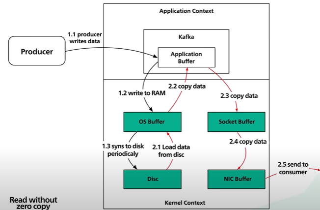
There are total of 4 copy of data and 2 system calls. Not efficient.
Kafka with zero copy.
The data page id loaded from the disk to the OS cache. With zero copy Kafka uses the system call called sendfile() to tell the OS to copy the data from the OS cache to the NIC buffer.
In the process the only copy is from the OS cache to the NIC buffer.
In the modern network card it is done by DMA - Direct Memory Access. DMA used and CPU is not involved and the process is efficient.
Sequential IO and DMA and zero copy principle are the corner stone of the Kafka high performance.
How to store password in the database.
Password is not stored in plain text anyone having the database access can easily read the password.
Open Web Application Security Project - OWASP provides some guidelines on how to store password.
Using modern Hashing function. It is one way it is impossible to decrypt hash.
There are some common legacy hashing function like MD5, SHA-1 are fast. They are less secure and should not be used.
Another way - SALT the password meaning add a unique random generated string in each password as a part of hashing process. Attackers will access the password using a technique called rainbow tables and database locks hacker can crack the password in seconds.
Password provided by the user and then added a randomly generated salt and then you make a hash function and value of this entire thing. The hash is stored in the database along with the salt.
Bare Metal, Virtual Machines and Container.
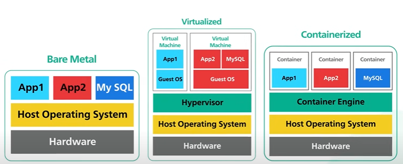
Bare metal server is a computer that is a single tenant only. Bare metal gives all the hardware resources and the software to run. Bare metal server are physically isolated and the isolation helps in not getting impacted by one network bandwidth with the other high CPU use.
Bare metal is expensive hard to manage hard to scale.
Virtual machine is an emulation of a physical computer. Virtual machine run on a single piece of a bare metal hardware On top of that there is the host operating system and on top of that there is a special software known as the hypervisor.
Hypervisor monitors the virtual machine it creates a layer over the hardware so that multiple operating system can run along side each other. Each virtual machine has its own guest OS. On top of the operating system runs the application.
Bare Metal Hypervisor is different that Bare Metal Hardware.
Bare metal hypervisor controls the hardware directly with relying on the host operating system. It gives the hypervisor full control over the hardware and provide high performance.
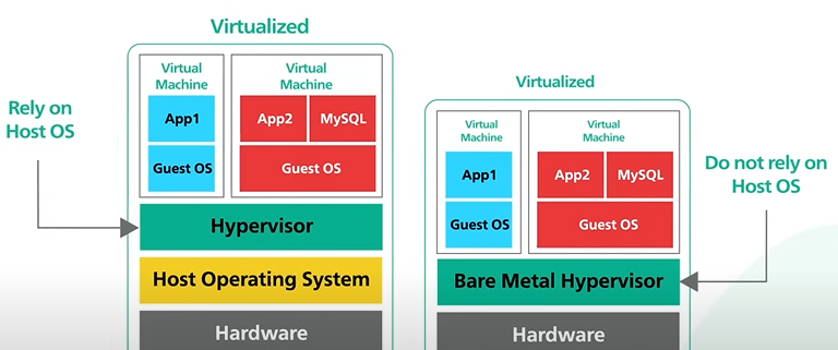
Hardware that supports Bare metal hypervisor are expensive.
Virtual machines are cheaper to run and share the same hardware allowing much high resource utilization.
Virtual machine is vulnerable for the noisy neighbor problem where one system and application will get impacted by other system being using 100% CPU or 95% network bandwidth. Virtual machine running on the same bare metal hardware shares the same physical cpu core which makes it vulnerable for any attacks.
Container is a lightweight and standalone application with all its dependencies. Continuation is a lightweight version of virtualization.
Here there is a bare metal hardware with a host operating system But instead of virtualizing the hardware with the hypervisor like in virtualization we virtualize the OS with a special software called the container engine. On top of this container engine they run the container which is an individual applications isolated from each other.
Containers is scalable and portable and there are lightweight to run on the virtual machine. A Bare Metal server can hold more Containers than virtual machines. Containers are easy to deploy.
They share the same underlying operating system and the isolation are the operating system level. Containers are exposed to wider class of security vulnerability.
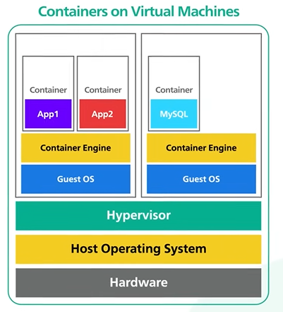
We can run containers inside the Virtual machine and it will increase the security.
After container there is the serverless and edge computing. The server less architecture using the GCP AWS.
Design a location Based System - Yelp.
Designing a proximity service meaning designing the best restaurant nearby or mapping to the closest gas station.
Functional requirement.
Given a user location in the search radius as input. Return all businesses within the search radius.
Business owner can add delete update a business. The changes doesnt need to be real time it can appear after one day.
User can view the details of the businesses in that page.
Non-functional requirement.
DAU - 100M.
Business - 200M.
The latency should be low users should be able to find the nearby businesses quickly.
The services should be highly available it should be able to handle traffic spikes during peak hours.
Assumptions.
DAU - 100M.
Business - 200M.
The daily active users are making around 5 queries per day.
100 Million DAU * 5 searches per user /100000 seconds in a day = ~5000.
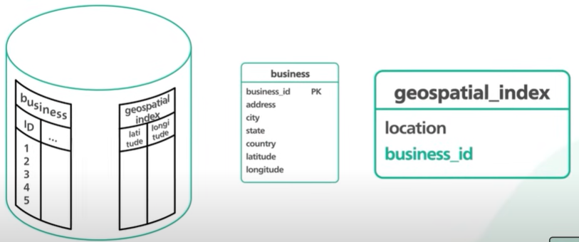
The database storage needed to store 200 million of data to estimate that we need to understand the schema design.
High-Level Design.
API design - Restful.
There were two broad api categories one to search the nearby businesses and one to get the details of the business.
GET /v1/search/nearby
|Field|Description|Type| |—-|—-|—-| |latitude|Latitude of a given location.|double.| |longitude|Longitude of a given location.|double.| |radius|Optional. Default is 5000 meters (about 3 miles)|int|
{
"total": 10,
"business": [{business object}]
}
We have shorten the api and can include pagination.
API to manage the business object.
GET /v1/businesses/:id Return detailed information about the business.
POST /v1/businesses Add a business.
PUT /v1/businesses/:id Update details of a business.
DELETE /v1/businesses/:id Delete a business.
The store required for the business table -
200 Million business * 1 KB = 200 * 10^6 * 1KB = 200GB.
The storage required for the nearby search table - 200 million * 24 bytes = ~ 5GB.
This database is very small so when the database is small then we can have wide variety of design and also we can use in memory database as well.
High Level Design.
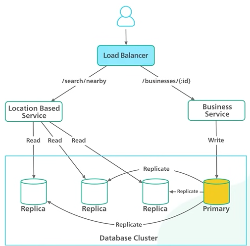
The load balance distributes incoming traffic across two services based on the api routes.
Boat services are stateless deploying stateless services behind a load balancer is a common design.
Company can use other setup to distribute traffic to services it could be envoy in a kubernetes cluster or API gateway on AWS.
The location based service has few characteristics -
Read heavy with no write request at all.
The QPS is high 5000 qps was our earlier estimate.
Service is stateless. It should be easy to scale horizontally.
The business service manages the business details and the qps of the update is not high.
In the recruitment we have understood the changes can reflect after sometime.
The read will be high and the qps is going to be high during peak hours. The data will not be changed frequently so it can be easily cache.
The system is read heavy.
Read qps is much higher than the writes qps.
The writes don’t need to be immediate.
On this observation we can say that the database cluster can be used with the primary secondary setup.
The primary database will be handling all the right requests and the read replica handles the heavy read request.
Twitter will be first stored into the primary and then it will be replicated to the other database there can be a bit of delay in the updated and consistent data but again the changes does not need to be reflected in real time.
Design Deep Dive.
Database to do the location based search - Geospatial database store and query data in geometric space like location data. Some example of these type of data are Redis GEOHASH and Postgres PostGIS extension.
Understanding how the db works - discuss the common algorithm behind the geospatial index that powers the database.
Intuitive and inefficient way - Draw a circle and find the businesses within the circle.
SELECT business_id, longitude, latitude
FROM business
WHERE (latitude
BETWEEN {:my_lat} - radius AND {:my_lat} + radius)
AND
(longitude BETWEEN {:my_long} - radius AND (:my_long} + radius)
The query is not efficient and it search in 200M data.
One way to index the latitude and longitude. Data returned for each dimension is huge. We can retrieve all businesses within a latitude range or longitude range.
To fetch businesses within a search radius we need to find the intersection of those ranges. It is inefficient and each dataset contains a lot of data.
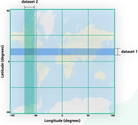
The problem with this approach is the index can increase the search in one of the two dimensions.
The follow up is can we map two dimension data into one dimension so we can build a single index on it.
There are 2 approaches in Geospatial indexing - Hash.
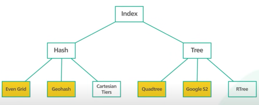
One way - evenly divide the grid and get the business within the grid. The problem is in few area the return of the businesses will be high and in few areas the business are low.

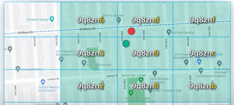
Geohash helps as it stores the two dimensional data into an one-dimensional string of letters and digits. It divides in four quadrant along the prime meridian and equator. Four quadrants are represented by two bits.

Each part is again divided into grids. The bits in the sub-grids are appended to the existing bits.
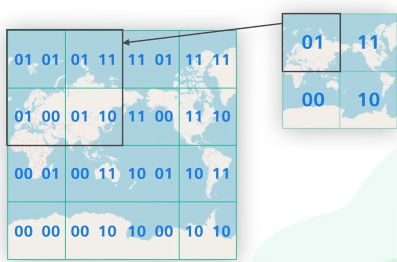
It repeats the subdivision and keeps adding more bits to the Geohash. It stopped the subdividing when the sub grid reaches the specific size.
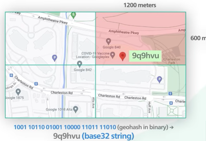
The example of a grid that contains the Google headquarter Institute of a long one and zero to represent the Jio hash design coded in a base 32 string.
The base32 string shows the size of the grid the idle size should be 4 5 or 6. If the value is higher than 6 then the grid size is too small and if it is less than 4 then the grid size is too big.
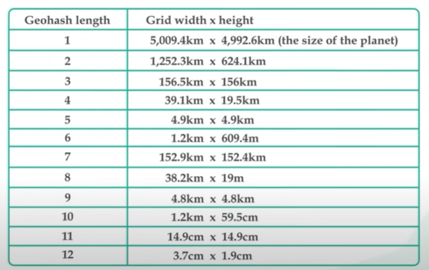
How do we choose the right precision given a search radius?
We find the minimal geohash length that covers the whole circle. For example if the radius is 2 km the Geohash length should be 5.
Another property Geohash is a string and searching all business within a geohash is very simple.
There are some cases when did you hash might not work properly. These edge cases have to do with how the boundaries are handled.
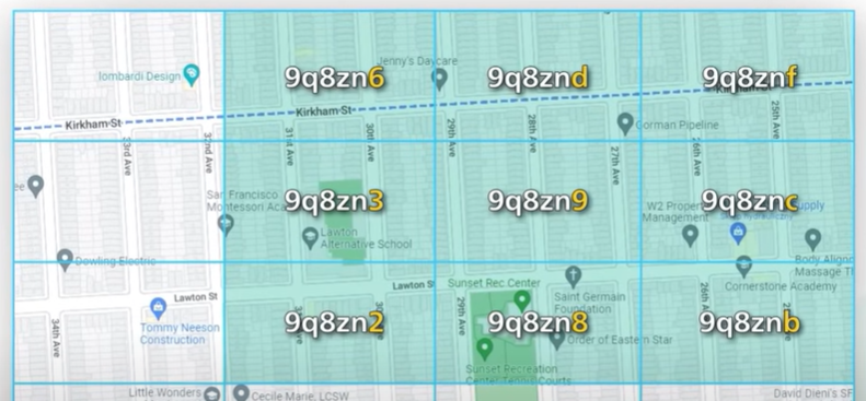
When two geohash strings share a long prefix we know they are close. The grid 9q8zn shares the same prefix.
The reverse is not true. Two places could be right next to each other but have no shared prefix a the grid on the either side of the equator or the prime meridian are in different halves of the world. Example two cities in France can be nearby but they are not sharing any common prefix.
Another boundary issue can be the two locations can have long shared prefix but they are in different geohash.
The common solution to bowl of these issues to fetch businesses is not only within the current date but also 8 grids surrounding it.
Calculating the neighboring geohash is easy and done in constant time using the library.
Implementing the location best service using a tree based indexing.
The common tree index is quadtree and googles2.
QuadTree.
A Quadtree data structure that partition a two dimensional space by recursively subdividing it into 4 quadrants.
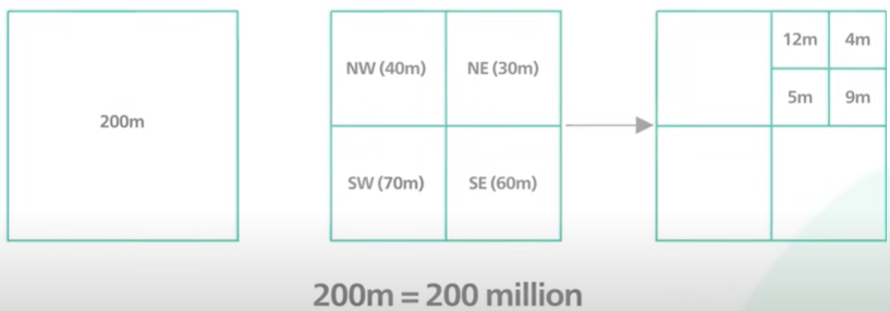
The subdivision stops when the greet meets certain criteria.
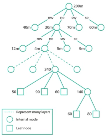
In out case the criteria can be keep dividing unto the number of businesses in a great his no more than similar say 100.
A keyboard for Quadtree or any other tree-base index is that it is an in memory data structure and not a database solution.
It means that the index is built by our own code and runs on the location-based servers.
We use the Geohash as the geospatial index to speed up the location search.
How do we structure the geospatial_index table?
It should contains two columns - geohash and business Id. Any relational db can handle geohash. The Geohash column contains the geohash of the right precision for each business.
Converting the latitude and longitude to the geohash is easy and libraries can do it.

Two things we should discuss with the table schema - Many business would share the same geohash. It means different business Ids within the same Geohash are stored in different database rows. The geohash and business id columns together form a compound key.
With the compound key, it makes the removal of a business from the table efficient.
In our application we are only interested in the geohash with precisions 4 to 6. They correspond to different search radii from 0.5km to 20 km.
The geohash column will all have the precision of 6. We use the LIKE operator in SQL to search for shorter prefix length.
Using the query we find everything that is within the geohash of ‘9q8zn’.
Scale the geospatial index table.
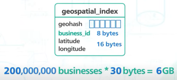
We do not need to scale more than one db table. The column geohash is 6 bit long and business_id is 64 bit like 8 bytes. We can also store the latitude and longitude so it is easy to calculate the distance of each business from the user and its about 16 bytes. Each row is 30 bytes.
200 million business the data is 6GB.
The database can be fit inside one server the read QPS is 5000 which is quite high.
The single db not have enough CPI or network bandwidth to handle all the read request.
Increase the speed of read there are two ways - Read replica or sharding.
Sharding is complex. It requires sharding logic in application layer. In the application entire database can be in a single machine there is no reason to use shard.
The better approaches to use the read replica of the geospatial_index table to help the read load.
Do we need a caching model in our design?
Our workload is read heavy and the Geospatial data set is small.
The read performance is bottlenecked then we can use read replicas.
There is another dataset to design - business table.
The data set for the business table with 200 million businesses is in terabyte range. Modern hardware can perform it. The dataset size is on the borderline where sharding might make sense.
The update rate is low and the db is read heavy. We should be able to get away without sharding if we put a cache in front of it.
The cache will take most of the read load of the frequently accessed businesses and it should give the business table quite a bit of headroom to grow.
There are a lot of options for the business table and first one is to use single table and get the product grows and with the help monitoring we can react to the growth and usage pattern and decide later to either shard or add more read replicas or add cache in front of it.
Search workflow.
Bob tries to find the restaurant within 500 meters. The client sends the location and search radius to the load balancer.
The load balancer forward the request to the location based service.
Based on the location and search radius, the service finds the Geohashes precision that matches the search request.
500 meter maps to the geohash length of 6.
This service calculates the neighbouring Geohash. There will be a total of 9 Geohash to query against the geospatial index table.
The service sends a query to the database to fetch the business ids and the latitude and longitude pairs within those geohashes.
The service uses the latitude and longitude pair to calculate the distance between the user and the businesses and rank it and return the business to the client
UPI scan and pay.
https://youtu.be/XS8ACikD2qs?si=dt6TPUUopLTV4agv
This method of payment is available via digital wallet apps like Paytm, PayPal and Venmo by scanning a dynamically generated QR code at the point of sale terminal. How does it work? Let’s take a look. To understand how it works, we need to divide the “Scan To Pay” process into two parts. The first part is for the merchant to generate a QR code and display it on screen. The second part is for the consumer to scan the QR code and pay. Let’s take a look at the steps for generating the QR code. When we’re ready to pay, the cashier clicks the checkout button. The cashier’s computer sends the total amount and order ID to the payment service provider. The PSP saves this information to the database and generates a QR code URL. The PSP returns the QR code URL to the cashier’s computer. The cashier’s computer sends the QR code to the checkout terminal. The checkout terminal displays the QR code. All these steps complete within a second. Now the consumer pays from the digital wallet by scanning the QR code, and here are the steps involved. The consumer opens the digital wallet app and scans the QR code. The total amount to pay is displayed in the app after confirming the amount. The consumer clicks the pay button. The wallet app notifies the PSP that the given QR code has been paid. The PSP marks the QR code as paid and returns a success message to the wallet app. The PSP notifies the merchant that the consumer has paid the given QR code. This is how to pay using a dynamic QR code. It is dynamic because the QR code is generated for one-time use. It is also possible to pay by scanning the printed QR code at the merchant. This is called static QR code. It works a bit differently and we might cover it in a different video. If you would like to learn more about system design, check out our books and weekly newsletter. Please subscribe if you learned something new. Thank you so much, and we’ll see you next time.
Consistent Hashing.
Data distributed across multiple server and it is horizontal scaling.
Data should be evenly distributed in the server and can be done by hash function.
ServerIndex = hash(key) % N. N number of server.
Hash function return same value for the same key. When the number of server is same the hash function will return the same value for the key.
When the number of server change like the reduced or increased then the data stored in the server is arranged to other server. The new hash function will return new value.
Consistent Hashing main purpose is all object to stay assigned to the same server even as the number of object changes. Hashing the object key and also the server name. The object and the server name are used into the same hashing function to the same range of values.
There is an array of x0 to xN and it is a hash range and the end of the array are connected making a circle.
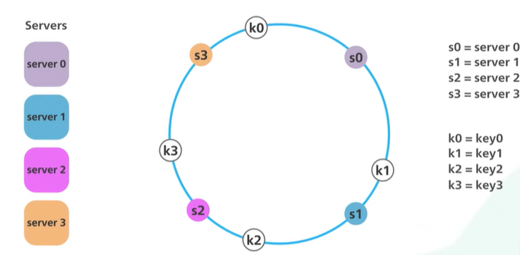
The hash is used to map the data into the ring. The modulo is not used.
To locate the server for a particular object we go clock wise from the location of the object in the ring until a server is found.
k0 to s0, k1 to s1.
Another server added then only k0 will be mapped to s4. The other key are in their place.
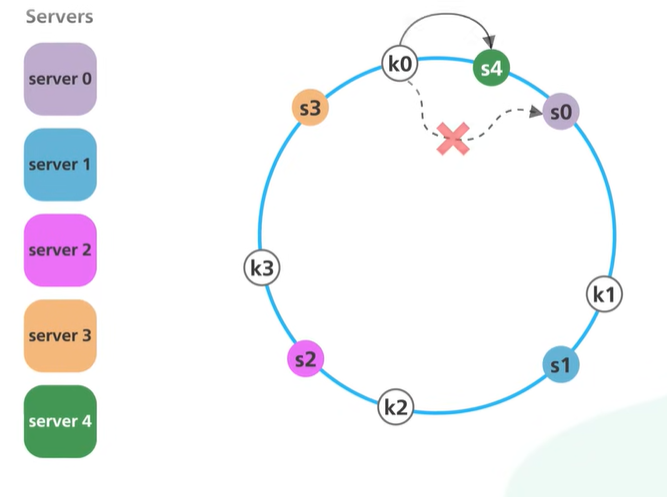
With simple hashing when a new server is added almost all keys need to be remapped. With consistent hashing adding a new server only requires redistribution of a fraction of the key.
Drawbacks - When all server in a same place then all data will come to the same server.
When one server removed then the entire load come to the next server.
Virtual node helps in it and one server present multiple location in the ring. Each location represents the server in the ring.
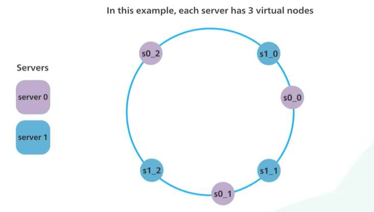
The virtual node will be managed by the s0 and s1.
More virtual node the data is more balanced.
More virtual node meaning more storage to store the metadata of the virtual node.
NoSQL db like Amazon Dynamo DB and Apache Cassandra uses consistent hashing for the data partitions.
CDN uses Consistent Hashing to distribute the web content evenly among the server.
Load Balancer like Google Load Balancer use Consistent hashing to distribute persistent connections evenly.
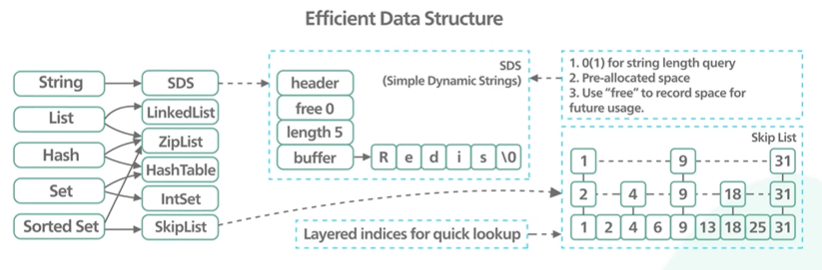
Why Redis fast?
Reddit is a very popular in memory database.
Redis uses RAM and not disk.
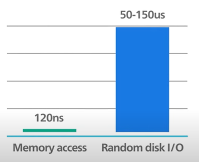
Memory access is faster than Random disk IO.
Pure memory gives the axis of high read and write throughput and low latency and the trade off is the data set cannot be larger than memory.
Code wise in memory data structure is far more easy to implement than on disk.
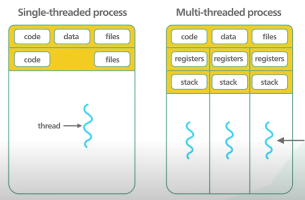
Another reason Redis is fast because it is single threaded.

Multi threaded application requires locks and other synchronisation mechanism.
How does single threaded code base handle thousands of requests incoming and outgoing ? Won’t the thread gets block waiting for each request to get complete individually?
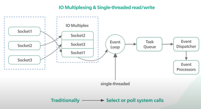
It’s the male function of the IO multiplexing. In multiplexing operating system allows a single thread to wait on many sockets.
On Linux the Epoll is a performant variant of IO multiplexing that support thousands of connection in constant time.
One drawback of the single threaded design is that it does not leverage all the CPU course available into this modern hardware system.
Another reason of red is being fast is that it can use the low level data structure like linked list, HashTable and Skiplist without being thinking about how to persist them to the disk efficiently.
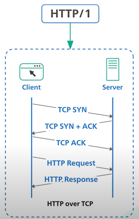
HTTP1 HTTP2 HTTP3.
HTTP1.
Every request to the same server requires a separate tcp connection.
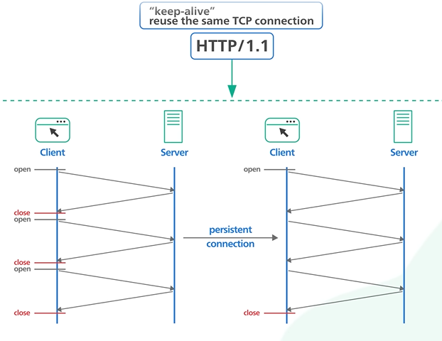
HTTP 1.1
Followed the same TCP connection. It follows the “keep-alive” mechanism and reuse the same tcp connection so that the connection can be used for more than a single request.
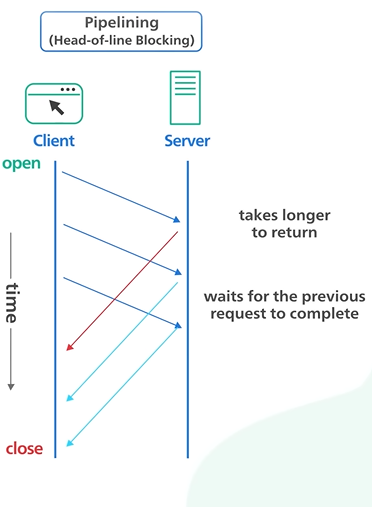
HTTP 1 .1 allowed the HTTP pipelining. It allows client to send multiple request before waiting for each response.
The response must be received in same order as it is send. It was tricky to maintain and the support removed from many servers.
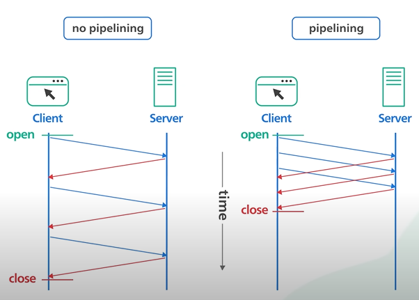
When one packet lost all subsequent request are impacted.
HTTP 2 each comes in stream. It solves the Head of line issue in the application layer but the issue still exists in the Transport layer.
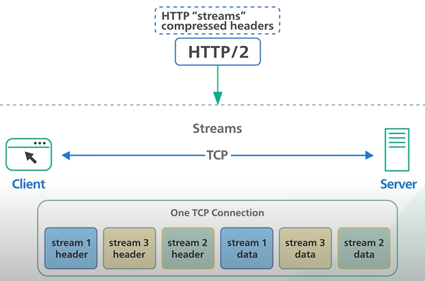
HTTP 2 introduces the PUSH capability to the server when the client new data is available without the client to poll.
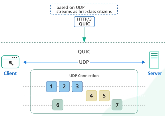
HTTP 3 uses QUIC protocol in the transport and not the TCP. It is based on UDP and consider stream as the first class citizen.
QUIC stream shares the same quic connection so no handshake required. It delivers independently and packet loss will not effect others.
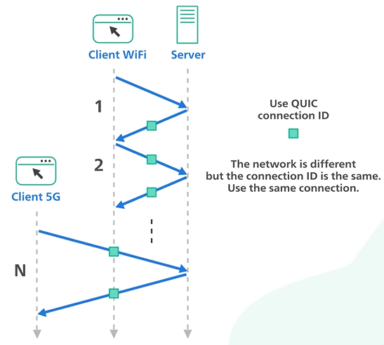
The QUIC uses the Connection Id and the connection to move from the IP address and network quickly.
What is REST API.
API stands for Application Programming Interface. It is a way for two computers to talk to each other. The common API standard used by most mobile and web applications to talk to the servers is called REST. It stands for REpresentational State Transfer.
It is a new set of rules that has been the common standard for building web API since the early 2000s. An API that follows the REST standard is called a RESTful API.
Rest Api Rules - Uniform Interface, Client-Server, Stateless, Cacheable, Layered System, Code on Demand.
A RESTful API organizes resources into a set of unique URIs, or Uniform Resource Identifiers. The URIs differentiate different types of resources on a server.
Here are some examples. The resources should be grouped by noun and not verb.
An API to get all products should be /products and not /getAllProducts.
A REST implementation should be stateless. It means the two parties don’t need to store any information about each other, and every request and response (cycle) is independent from all others.
There are two final points to discuss to round out a well-behaved RESTful API.
If an API endpoint returns a huge amount of data, use pagination. A common pagination scheme uses “limit” and “offset” as parameters.
Example - products?limit=25&pffset=50
Versioning of an API is very important. Versioning allows an implementation to provide backward compatibility, so that if we introduce breaking changes from one version to another, consumers can get enough time to move to the next version.
The most straightforward is to prefix the version before the resource on the URI v1/products.
There are other popular API options like GraphQL and gRPC.
NOSQL LSM Tree.
NoSQL Database like Cassandra became very popular. The secret sauce for the NoSQL Db is the Log Structure Merge Tree.
LSM Tree is optimized for fast write.
How data is store in a relational Database.
In relational database cities generally done by B Tree and B Tree is optimized for reads.
Updating the B Tree relative to expensive as it involves random IO and include updating multiple pages on disk. It limit how fast a B Tree can ingest data.
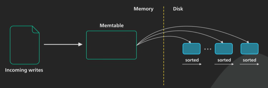
LSM works differently, writes are batched in memory as they arrive in a structure called a memtable. A memtable is ordered by object key and is usually implemented as a balanced binary tree.
As a memtable reaches a certain size it is flushed to disk as an immutable Sorted String Table.
An SSTable store the key value pair in a sorted sequence. The write are all sequential IO. Fast on any storage media.
The new SSTable becomes the most recent segment of the LSM tree as more data comes in more and more of this immutable SSTable are created and added to the LSM tree. Each one representing a small chronological subset of the incoming changes.
Since SSTable is immutable and update to an existing object key does not overwrite an existing SSTable.
Instead a new entry is added to the most recent SSTable which supersede any entries in the old access table for the objective.
Deleting an object in SSTable we cannot mark anything in the sustainable as deleted. To perform a delete it adds a marker called a tombstone to the most recent SSTable for the object key.
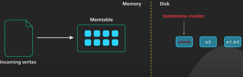
When we get the tombstone on read we known that the object has been deleted. It is a bit unintuitive that a delete takes up extra space.
To serve a read request we first try to find the key in the memtable then in the most recent SSTable in the LSM tree then the next SSTable.
Since the sustainability sorted the lookup can be done efficiently.
The number of SSTable grows it would take an increasingly long time to look up a key. As the SSTable accumulate the more outdated entries as keys are updated and tombstones are added. It takes disk space.
To fix the issues there is a periodic merging and compaction process running in the background to merge SSTable and discard outdated or deleted values.
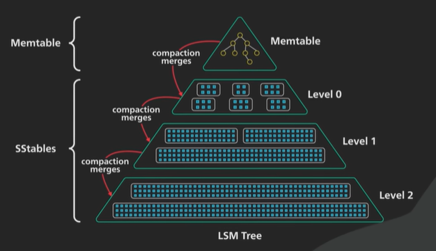
SSTable is sorted so the merging and compaction process is simple and uses mergesort algorithm.
When SSTable are merged they are organized into labels. There are different strategies to determine where and how the SSTable are merged and compacted.
There are two board strategies Size tiered compaction and level compaction.
Size tiered compaction - Cassandra is optimized for write throughput.
Level compaction - Rock DB is more read-optimized.
Complexion keeps the SSTable manageable. This is similar organised in levels.
Each table gets larger as SSTable from the level above are merged into it.
Compaction contains a lot of IO.
A mistuned compaction could starve the system and slow down both read and write.
Optimization for the LSM tree.
There are many optimizations which tries to perform the read operations similar to the B Tree.
It look up on every label of the SSTable. searching is easy as it is done on the sorted data but then going through all of the data takes a lot of IO.
Many system contains a summary table in each level which contains the min max range of each disc block of every level.
Another issue to look up a key that does not exists. It looks all the eligible bocks in all the levels. Most system keeps a bloom filter at each level.
A bloom filter is a space efficient data structure that returns a firm no if the key does not exist. It help the system not to look at each level and it improves the IO system.
Bloom Filters.
Bloom Filter is a space efficient probabilistic data structure.
It would answer with a firm no and probably yes.
Use case can tolerate some false positives but not any false negatives a bloom filter could be very useful.
We cannot removes an item from a bloom filter it never forgets.
NoSql databases use bloom filter to reduce disk read for keys that don’t exist. An lsm tree based database searching for a key that doesn’t exist requires looking through many files and it’s very costly.
CDN like Akamai use bloom filter to prevent caching one-hit-wonders these are web pages that are only requested once.
Akamai data 75% of the pages at one-day-wonders using a bloom filter to track all the urls seen and only caching a page on the second request is significantly reduces the caching workload and increases the caching hit rate.
Web browsers like chrome used to use a bloom filter to identify malicious url. Urls was first checked against a bloom filter. It only performed a more expensive full cheque of the url if the bloom filter returned a probably yes answer. This is no longer used however as the number of malicious urls grows to the millions and a more efficient but complicated solution is needed.
Some password validators use bloom filter to prevent users from using weak passwords sometimes it’s wrong password will be a victim or a false positive.
The critical ingredient to a good bloom filter is some good hash functions these hash functions should be fast and they should produce outputs that evenly at randomly distributed, few collisions can be there.
A bloom filter is a large set of buckets where each bucket containing a single bit and they all start with zero.
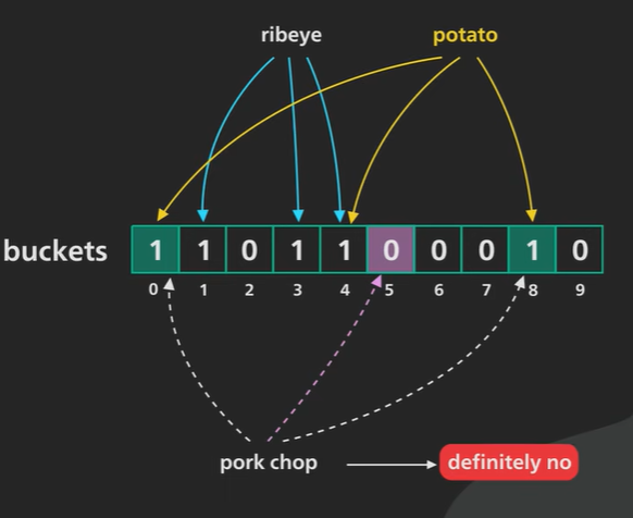
Example to keep track of the food liked for this example we’ll use a bloom filter with 10 buckets (0-9) and we’ll use three hash functions.
Putting ribeye into the bloom filter the three hash functions return the numbers 1 3 4 these were set the buckets to one.
Potato into the boom filter the hashing function returned to number 0, 4, 8 this time set the value to 1.
Ask bloom filter about ribeye since the same input always hashes to the same output ribeye still hashes to the number 1, 3, 4 bloom filter array value 1. Correct.
Asking about chop the value of the hash say 1, 5, 8 and the value 5 is not 1 in the array so the answer is no and it is correct.
Asking lemon and the hash return 1, 4, 8 and the value are 1 in array and then search happen and lemon not present. It say yes but the value not present. It is a false positive case.
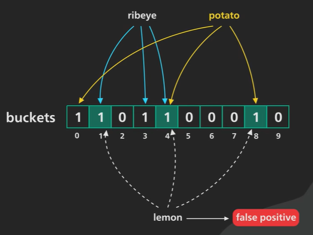
The hash function should be good and the size of the array should be proper to avoid less false positive.
Back Of Envelope Estimation.
https://youtu.be/UC5xf8FbdJc?si=QUtv6DCN5ACTBzoE
Back-of-the-envelope math is a very useful tool in our system design toolbox. In this video, we will go over how and when to use it, and share some tips on using it effectively. Let’s dive right in. Experienced developers use back-of-the-envelope math to quickly sanity-check a design. In these cases, absolute accuracy is not that important. Usually, it is good enough to get within an order of magnitude or two of the actual numbers we are looking for. For example, if the math says at our scale our web service needs to handle 1M requests per second, and each web server could only handle about 10K requests per second, we learn two things quickly: One, we learn that we will need to cluster of web servers, with a load balancer in front of them. Two, we will need about 100 web servers. Another example is if the math shows that the database needs to handle about 10 queries per second at peak, it means that a single database server could handle the load for a while, and there is no need to consider sharding or caching for a while. Now let’s go over some of the most popular numbers to estimate. The most useful by far is requests per second at the service level or queries per second at the database level. Let’s go over the common inputs in a requests-per-second calculation. The first input is DAU, or Daily Active Users. This number should be easy to obtain. Sometimes, the only available number would be Monthly Active Users. In that case, estimate the DAU as a percentage of MAU. The second input is the estimate of the usage per DAU of the service we are designing for. For example, not everyone active on Twitter makes a post. Only a percentage does that. 10%-25% seems to be reasonable. Again, it doesn’t have to be exact. Getting within an order of magnitude is usually fine. The third input is a scaling factor. The usage rate for a service usually has peaks and valleys throughout the day. We need to estimate how much higher the traffic would peak compared to the average. This would reflect the estimated requests-per-second peak where the design could potentially break. For example, for a service like Google Maps, the usage rate during commute hours could be 5 times higher than average. Another example is a ride-sharing service like Uber, where weekend nights could have twice as many rides as average. Now, let’s go over an example. We will estimate the number of Tweets created per second on Twitter. Note that these numbers are made up, and they are not official numbers from Twitter. Let’s assume Twitter has 300 million MAU, and 50% of the MAU use Twitter daily. So that’s 150 million DAU. Next, we estimate that about 25% of Twitter DAU make tweets. And each one on average makes 2 tweets. That is 25% * 2 = 0.5 tweets per DAU. For the scaling factor, we estimate that most people tweet in the morning when they get up and can’t wait to share what they dreamed about the night before. And that spikes the tweet creation traffic to twice the average when the US east coast wakes up. Now we have enough to calculate the peak tweets created per second. We have: 150 million DAU times 0.5 tweet per DAU, times 2x scaling factor divided by 86,400 seconds in a day. That is roughly about 1,500 tweets created per second. Let’s go over the techniques to simplify the calculations. First, we convert all big numbers to scientific notation. Doing the math on really big numbers is very error-prone. By converting big numbers to scientific notation, part of the multiplication becomes simple addition, and division becomes subtraction. In the example above, 150 million DAU becomes 150 times 10 to the sixth or 1.5 times 10 to the eighth. There are 86,400 seconds in a day, we round it up to 100,000 seconds, and that becomes 10 to the fifth seconds. And since it’s a division, 10 to the fifth 5 becomes 10 to the minus fifth. Next, we group all the power of tens together, and then all the other numbers together. So the math becomes: 1.5 times 0.5 times 2 And 10^8 * 10 ^(-5) = 10^(8-5) = 10^3 Putting it all together, it’s 1.5x10^3, or 1,500. Now with practice, we should be able to convert a large number to scientific notation in seconds. And here are some handy conversions we should memorize: As an example, we should know by heart that 10^12 is a trillion or a TB, and when we see a number like 50TB, we should be able to convert it quickly to 5x10^1x10^12, which is 5x10^13. We are going to ignore the fact that 1KB is actually 2^10 bytes, or 1,024 bytes, and not a thousand bytes. We don’t need that degree of accuracy for back-of-the-envelope math. Let’s wrap up by going through one last example. We’ll estimate how much storage is required for storing multimedia files for tweets. We know from the previous example that there are about 150M tweets per day. Now we need an estimate on a percentage of tweets that could contain multimedia content, and how large those files are on average. With our meticulous research, we estimate that 10% of tweets contain pictures, and they are about 100KB each, and 1% of all the tweets contain videos, and they are 100MB each. We further assume that the files are replicated, with 3 copies each, and that Twitter would keep the media for 5 years. Now here is the math. For storing pictures, we have the following: 150M tweets x 0.1 in pictures x 100KB per picture x 400 days in a year x 5 years * 3 copies So, that turns into: 1.510^8 x 10^(-1) x 10^5 x 4x10^2 x 5 x 3 Again, we group the powers of tens together. This becomes: 1.5 times 4 times 5 times 3, which is 90 and 10 to the (8-1+5+2), which is 10^14 And that becomes 9x10^15, which is, from the table, 9 PB. For storing videos, we take yet another shortcut. Since videos on average are 100MB each while pictures are 100KB, a video is 1000 times bigger than a picture on average. Second, only 1% of tweets contain a video, while pictures appear in 10% of all the tweets. So videos are one-tenth as popular. Putting the math together, the total video storage is 1000 x 1/10 of picture storage, which is 100 x 9PB, or 900 PB. In conclusion, back-of-the-envelope math is a very useful tool in our system design toolbox. Don’t over-index on precision. Getting within an order of magnitude is usually enough to inform and validate our design. If you would like to learn more about system design, check out our books and weekly newsletter. Please subscribe if you learned something new. Thank you so much, and we’ll see you next time.
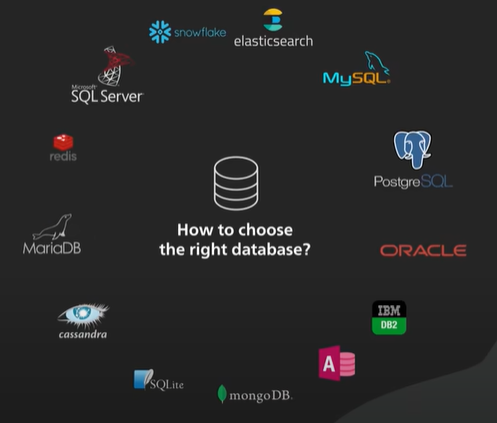
Choose right DB.
How does live streaming platform work.
https://youtu.be/7AMRfNKwuYo?si=cOzaxorGjuqwkeWd
How do these popular live streaming platforms deliver video content from the streamer’s computer to the viewer’s device, or the so-called “glass-to-glass” latency, that is measured in low tens of seconds or faster? Let’s take a look. Live streaming is challenging because the video content is sent over the internet in near real-time. Video processing is compute-intensive. Sending a large volume of video contents over the internet takes time. These factors make live streaming challenging. Let’s take a look at how a video stream goes from the streamer to the viewers. First, the streamer starts their stream. The source could be any video and audio source wired up to an encoder, something like the popular open-source OBS software. Some popular platforms like YouTube provide easy-to-use software to stream from a browser with a webcam, or directly from a mobile phone camera. The job of the encoder is to package the video stream and send it in a transport protocol that the live streaming platform can receive for further processing. The most popular transport protocol is called RTMP, or Real-time Messaging Protocol. RTMP is a TCP-based protocol. It started out a long time ago as the video streaming protocol for Adobe Flash. The encoders can all speak RTMP, or its secure variant called RTMPS. There is a new protocol called SRT, or Secure Reliable Transport, that could start to replace RTMP. SRT is UDP-based and it promises lower latency and better resilience to poor network conditions. However, most of the popular streaming platforms do not yet support SRT. To provide the best upload condition for the streamer, most live streaming platforms provide point-of-presence servers worldwide. The streamer connects to a point-of-presence server closest to them. This usually happens automatically with either DNS latency based routing or an anycast network. Once the stream reaches the point-of-presence server, it is transmitted over a fast and reliable backbone network to the platform for further processing. At the platform, the main goal of this additional processing is to offer the video stream in different qualities and bit-rates. Modem video players automatically choose the best video resolution and bit rate based on the quality of the viewer’s internet connection and can adjust on the fly by requesting different bit rates as the network condition changes. This is called adaptive bitrate streaming. The exact processing steps vary by platform and the output streaming formats. In general, they fall into the following categories. First, the incoming video stream is transcoded to different resolutions and bit-rates - basically different quality levels for the video. The transcoded stream is divided into smaller video segments a few seconds in length. This process is called segmentation. Transcoding is compute-intensive. The input stream is usually transcoded to different formats in parallel, requiring massive compute power. Next, the collections of video segments from the transcoding process are packaged into different live streaming formats that video players can understand. The most common live-streaming format is HLS, or HTTP Live Streaming. HLS was invented by Apple in 2009. It is the most popular streaming format to date. An HLS stream consists of a manifest file, and a series of video chunks, with each chunk containing a video segment as short as a few seconds. The manifest file is a directory to tell the video player what all the output formats are, and where to load the video chunks over HTTP. The resulting HLS manifest and video chunks from the packaging step are cached by the CDN. This reduces the so-called last-mile latency to the viewers. DASH, or Dynamic Adaptive Streaming over HTTP, is another popular streaming format. Apple devices natively do not support DASH. Finally, the video starts to arrive at the viewer’s video player. The “glass-to-glass” latency of around 20 seconds is normal. There are several factors a streamer or the live streaming platform could tune to improve this latency by sacrificing various aspects of the overall video quality. Some platforms simplify this tuning process by providing a coarse knob for the streamer to choose the level of interactivity they desire. The platforms then adjust the quality of the stream based on that input. This is largely a blackbox from the streamer’s perspective. The best thing the streamer could do is optimize their local setup for the lowest latency from the camera to the streaming platform.
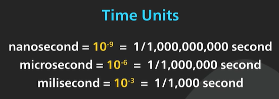
Latency Numbers.
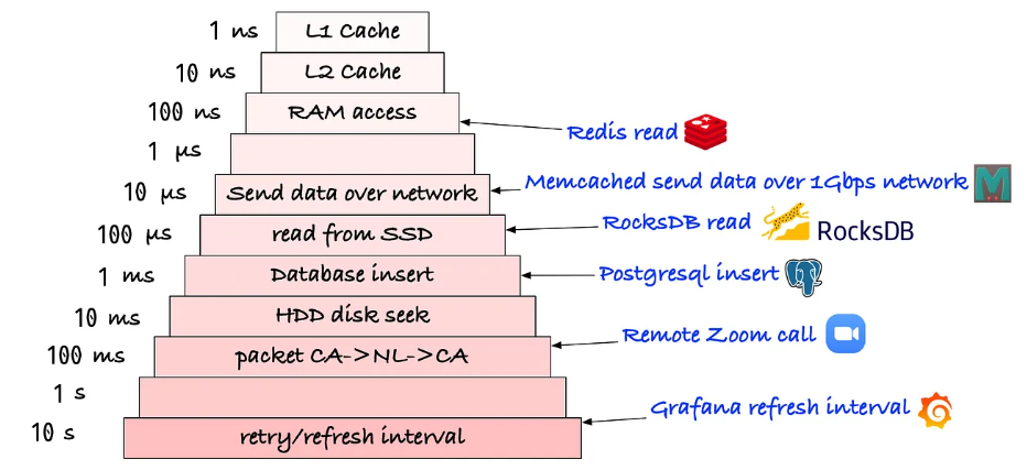
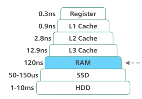
Disk access latency has improved HHD to SSD.
The network latency between countries has not improved as it covers the country and obeys the law of physics.
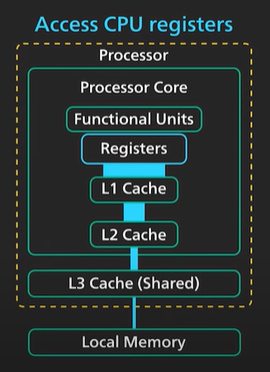
1 ns - Accessing CPU Register is sub-nanosecond range.
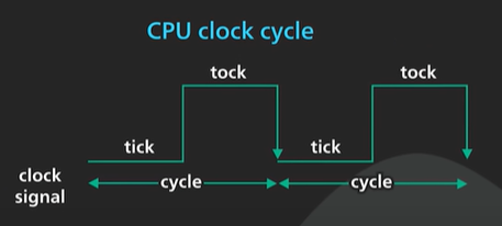
A clock cycle of a modern CPU is in sub-nanosecond range.
1-10 ns - L1 and L2 cache access. Some expensive CPU operations are in the range. Example like Branch Mispredict penalty can be 20 CPU clock cycle and it is in the range.
10-100 ns - L3 cache access is in the fast side of the range. For modern processor like Apple M1 referencing main memory is the slow end at the range.
Main memory access in modern CPU is 100 times slower than CPU register access.
100-1000 ns or 1 μs microsecond - System call. In linux making a simple system call takes several hundred nanoseconds. It is a direct call to trap into the kernel and back. It does not account the cost of executing the system calls.
It takes 200 ns to MD5 hash a 64 bit number.
1-10 μs - It is 1000 times slower than a CPU register access. Context switching in Linus thread takes few micro seconds.
10-100 μs - A network proxy like Nginx would take around 50 microsecond to process a typical http request. Reading 1 MB of data sequentially from a main memory takes around 50 μs. The read latency of SSD takes 100 μs to read 8k page.
100-1000 μs or 1 milliseconds - The SSD write latency is 10 times slower than read latency. Intrazone Network Round trip for modern cloud providers takes few hundred microseconds. A typical name cache already cache operation takes around 1 millisecond.
1-10 ms - Inter zone network round trip of clous takes this range. The seek time of the hard disk drive is about 5 ms.
10-100 ms - The network round trip between US East to US West Coast or the US East Coast and Europe is in this range. Reading of 1 GB sequential from main memory.
100-1000ms - The hash function becrypt is used to encrypt a password and it takes around 300 milliseconds. TLS handshake is in 250-500 ms range. It has several machine round trip so the number depends on the distance between the machines. The network round trip between the US West Coast and Singapore is in this range. Reading 1GB sequentially from SSD is also in this range.
1 s - Transferring 1GB over the network within the same cloud region takes about 10s.
What are Microservice.
https://youtu.be/lTAcCNbJ7KE?si=jMeNl8_zHMZxGxOV
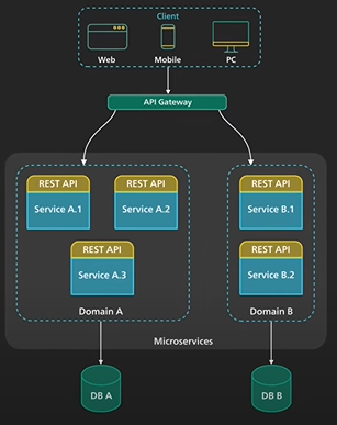
Microservices architecture enables large teams to build scalable applications that are composed of many loosely coupled services. What does a typical microservices architecture look like? And when should we use it? Let’s take a look. Microservices are loosely coupled. Each service handles a dedicated function inside a large-scale application. For example, shopping cart, billing, user profile, push notifications can all be individual microservices. These functional areas are sometimes called domains. Microservices communicate with each other via well-defined interfaces with small surface areas. The small surface areas limit the blast radius of failures and defects. It makes each service easier to reason about in the context of the entire application. Microservices talk to one another over a combination of remote procedure calls (RPC), event streaming, or message brokers. RPC like gRPC provides faster response, but the blast radius, or the impact to other microservices, would be larger when the service was to go down. Event streaming provides better isolation between services but they take longer to process. Microservices can be independently deployed. Since each service is small, easier to reason about, and has a smaller blast radius, this gives the operators peace of mind and confidence to deploy often. Microservices provide more flexibility to scale up individual microservices independently. The operational flexibility is invaluable. Well-architected microservices practice strong information hiding. This often means breaking up a monolithic database into its logical components and keeping each logical component well hidden inside its corresponding microservice. By logical component, it could mean a separate schema within a database cluster or an entirely separate physical database. This is an implementation detail. However, one big drawback of microservices is the breaking up of the database. By breaking up a database into separate logical units, the database can no longer maintain foreign key relationships and enforce referential integrity between these units. The burden of maintaining data integrity is now moved into the application layer. Let’s take a look at other critical components required for a successful implementation of microservices architecture. A key component is an API gateway. API gateway handles incoming requests and routes them to the relevant microservices. The API gateway relies on an identity provider service to handle the authentication and put authorization of each request coming through the API gateway. To locate the service to route an incoming request to, the API gateway consults a service registry and discovery service. Microservices register with this service registry and discover the location of other microservices through the discovery service. There are other useful components in a microservices architecture like monitoring and alerting, DevOps toolings for deployment, and troubleshooting, for example. Let’s wrap up by discussing when to use microservices architecture. Microservices cost money to build and operate. It really only makes sense for large teams. For large teams, it enables team independence. Each domain, or function, can be independently maintained by a dedicated team. In a well-designed microservices architecture, these independent teams can move fast, and the blast radius of failures is well-contained. Each service could be independently designed, deployed, and scaled. However, the overhead of a sound implementation is so large that it is usually not a good fit for small startups. One advice for startups is to design each function in the application with a well-defined interface. One day if the business and team are growing fast that microservices architecture starts to make sense, it would be more manageable to migrate. If you would like to learn more about system design, check out our books and weekly newsletter. Please subscribe if you learned something new. Thank you so much, and we’ll see you next time.
How Apple pay works.
https://youtu.be/cHv8LqkbPHk?si=dsTujVI2Ct1W28Nz
Which one is better? Let’s take a look. We’ll start by stating that both implementations are secure, but the technical details are a bit different. Apple Pay started in 2013. It was a novel idea then. It perfected the concept called tokenization where only a payment token representing the sensitive credit card info is needed to complete a purchase. It required close cooperation from payment networks like VISA and large issuing banks like JPMC to build a new system to support the wide adoption of payment tokens. Google Pay has been around since 2018. Before that, it was known as Android Pay, and before that, Google Wallet. The branding is confusing, and it appears that now Google Pay is Google Wallet again in some countries. We will refer to the current version that uses payment tokenization as Google Pay. Let’s take a look at how these systems work. Both platforms start by collecting sensitive credit card information on the device. It is worth noting that both platforms claim that they don’t store the PAN, or Primary Account Number, on the device itself. The PAN is then sent to the respective servers over HTTPS. At the Apple server, the credit card info is not stored anywhere. It is used to identify the payment network and the issuing bank for the credit card. To simplify, we will refer to the payment network like VISA and the bank that issues the credit card as the bank from here on out. The credit card info is then sent to the bank securely over the network. The bank validates the PAN and returns a token called DAN, or device account number. This number is uniquely generated for use only by the device. The generation of the DAN and the mapping of the DAN to the PAN is usually offloaded to a TSP, or a Token Service Provider. The TSP is where the most sensitive information lives. The DAN is then returned to the Apple server, and the server forwards the DAN to the iPhone where it is stored securely in a special hardware chip called Secure Element. Logically, the Apple server is just a pass-through. It is as if the iPhone directly sends the credit card info to the bank in exchange for the DAN. For Google Pay, this process is a bit different. Like Apple, the PAN is sent securely by the device to the Google server. The Google server uses the PAN to identify the bank. The PAN is then sent to the bank securely over the network. The bank validates the PAN and forwards it to the TSP for a payment token. The token is sometimes called DPAN, or Device PAN. The token is then sent back to the Google server, where it is forwarded to the device for safe storage. There are two points worth mentioning here that are different than Apple. One - The token is not stored in the Secure Element like on the Apple devices. It is stored in the wallet app itself. Two - Apple boasts to never store the payment tokens on its server. Google makes no such claim, and in fact, in its term of service, it states that payment information is stored on its server. We explained so far how each implementation turns the card info into some form of on-device payment token. Let’s take a look at how these tokens are used to make a purchase. For the iPhone, once we click Pay, the DAN is retrieved from the Secure Element and sent to the merchant’s Point-of-sale terminal over NFC, or Near Field Communication. This is really secure, because the DAN is sent directly from the Secure Element to the NFC controller on the device. The NFC controller and the Secure Element communicate with the point-of-sale terminal. The point-of-sale terminal sends the DAN to the merchant’s bank. The merchant’s bank identifies the payment network from the DAN and securely routes the DAN to the payment network. The payment network validates the DAN, then makes a request to the TSP to de-tokenize the DAN back to the original PAN. The PAN is sent securely from the TSP to the bank where the card was issued where the payment is authorized. For Google Pay, the flow is similar once the payment token reaches the point-of-sale terminal. How it gets from the device to the point-of-sale terminal is quite different. Android devices do not store the payment token in the Secure Element. It instead uses something called Host Card Emulation, or HCE. With HCE, the payment token is stored in the wallet app or retrieved at transaction time by the wallet app securely from the cloud. The NFC controller and the wallet app work together to transmit the payment token over NFC to the point-of-sale terminal. At that point, the rest of the transaction is the same as Apple’s. To conclude, both Apple Pay and Google Pay take advantage of the payment tokenization technology. Apple Pay perfected the technology and made it user friendly and secure. Google Pay’s implementation is similar. The main difference is how the payment token is stored, handled, and transmitted on device, and how the payment token could potentially be stored on the Google server. If you like our videos, you might like our weekly system design newsletter as well.
Proxy vs Reverse Proxy.
Nginx is called a reverse proxy.
There are 2 common types of proxy a forward proxy and reverse proxy.
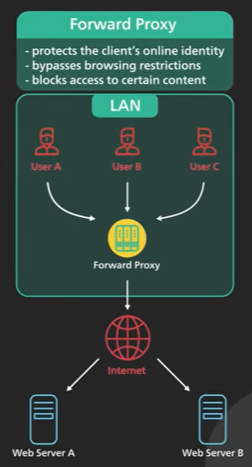
Forward proxy is a server and sits between a group of client machines and Internet. When those clients make request to websites on the Internet the forward proxy acts as a middleman intercepts those requests and talks to the web servers on behalf of those client machines.
Why do we do that?
There are a few reasons - Forward proxy protects the clients online identity, the ip address of the client is hidden from the server only the ip address of the proxy is visible it would be harder to trace back to the client.
Forward proxy can be used to bypass browsing restrictions. Some institutions the governments, schools and big businesses use firewalls to restrict access to the Internet by connecting to a forward proxy outside the firewalls the client machine can potentially get around these restrictions.
Forward proxy can be used to block access to certain content. It is not uncommon for schools and businesses to configure the networks to connect all clients to the web through the proxy and apply filtering rules to disallow sites by social networks.
Forward proxy normally requires a client to configure its application to point to it.
Large institutions they usually apply a technique called transparent proxies to streamline the process.
Transparent proxy works with layer 4 switches to redirect certain types of traffic to the proxy automatically there is no need to configure a client machines to use it.
It is difficult to bypass a transparent proxy when the client is on the institution’s network.
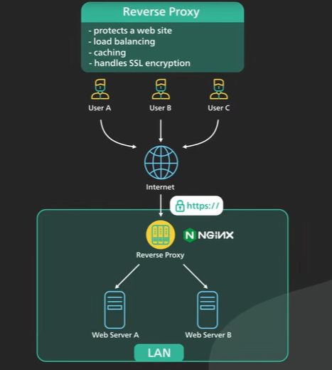
Reverse proxy sits between the Internet and the Web servers. It intercepts the reuqets from clients and talk to the server on behalf of the client.
Why would a website use a reverse proxy.
There are few good reasons.
A reverse proxy could be used to protect a website the website’s ip addresses a hidden behind the reverse proxy they’re not revealed to the clients this makes it much harder to target a ddos attack against a website.
A reverse proxy is used for load balancing a popular website handling millions of users every day is unlikely to be able to handle the traffic with a single server a reverse proxy can balance a large amount of incoming request by distributing the traffic to a large pool of web servers and effectively preventing any single one of them from becoming overloaded.
This assumes that the reverse proxy can handle the incoming traffic. Services like Cloudflare put reverse proxy servers in hundreds of locations all around the world this puts a reverse proxy closer to users and at the same time provides a large amount of processing capacity.
A reverse proxy caches static content a piece of content could be cached on the reverse proxy for a period of time if the same piece of content is requested again from the reverse proxy the locally cached version could be quickly.
The reverse proxy can handle ssl encryption ssl handshake is computationally expensive the reverse proxy can free up the origin servers from those expensive operations instead of handling ssl for all clients a website only needs to handle ssl handshake from a small number of reverse proxies.
Layers of Reverse Proc.
The first layer could be an edge service like Cloudflare. The reverse proxies are deployed to hundreds of locations worldwide closer to users.
The second layer could be an api gateway or load balancer at the hosting provider many cloud providers combine these two layers into a single ingress service.
The user will enter the cloud network at the edge closer to the user and from the edge the reverse proxy connects over a fast fibre network to the load balancer where the request is even a distributed over a cluster of web servers.
What is API Gateway.
https://youtu.be/6ULyxuHKxg8?si=H9Y7IPTtUgg3oKy9
API Gateway uses - Authentication and security policy enforcement, load balancing and circuit breaking, protocol translation and service discovery, monitoring, logging, analytics and billing, caching.
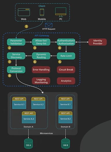
What does an API gateway do? Why do we need it? Let’s take a look. An API gateway is a single point of entry to the clients of an application. It sits between the clients and a collection of backend services for the application. An API gateway typically provides several important functions. Some common ones are: authentication and security policy enforcements, load balancing and circuit breaking, protocol translation and service discovery, monitoring, logging, analytics, and billing. And finally, caching. Let’s examine a typical flow of a client request through the API gateway and onto the backend service. Step 1 - the client sends a request to the API gateway. The request is typically HTTP-based. It could be REST, GraphQL, or some other higher-level abstractions. Step 2 - the API gateway validates the HTTP request. Step 3 - the API gateway checks the caller’s IP address and other HTTP headers against its allow-list and deny-list. It could also perform basic rate limit checks against attributes such as IP address and HTTP headers. For example, it could reject requests from an IP address exceeding a certain rate. Step 4 - the API gateway passes the request to an identity provider for authentication and authorization. This in itself is a complicated topic. The API gateway receives an authenticated session back from the provider with the scope of what the request is allowed to do. Step 5 - a higher level rate-limit check is applied against the authenticated session. If it is over the limit, the request is rejected at this point. Step 6 and 7 - With the help of a service discovery component, the API gateway locates the appropriate backend service to handle the request by path matching. Step 8 - the API gateway transforms the request into the appropriate protocol and sends the transformed request to the backend service. An example would be gRPC. When the response comes back from the backend service, the API gateway transforms the response back to the public-facing protocol and returns the response to the client. A proper API gateway also provides other critical services. For example, an API gateway should track errors and provide circuit-breaking functionality to protect the services from overloading. An API gateway should also provide logging, monitoring, and analytics services for operational observability. An API gateway is a critical piece of the infrastructure. It should be deployed to multiple regions to improve availability. For many cloud provider offerings, the API gateway is deployed across the world close to the clients.
What is GraphQL. REST vs GraphQL.
GraphQL is a query language for API developer by Meta.
It provides a scheme of the data in the api and user can ask what they need.
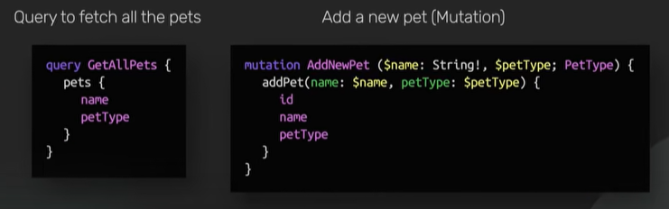
GraphQL sits between the clients and the backend services. It could aggregate multiple resource requests into a single query. It also supports mutations and subscriptions.
Mutations are GraphQL way of applying data modifications to resources.
Subscriptions are GraphQL way for clients to receive notification on data modifications.
GraphQL and REST both send HTTP request and receive HTTP response.
REST centers around resources each resource is identified by a url. It uses v3/books/123 to fetch a book from the bookstore api.
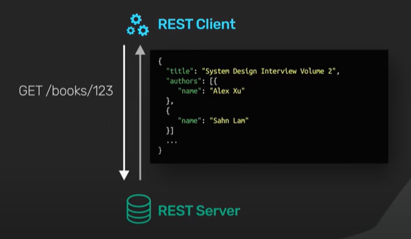
The authors field is implementation specific some rest api implementations by break them into separate REST call like /authors/3 or authors/5
In GraphQL it looks different we first define the types in this example we have the book and author types.
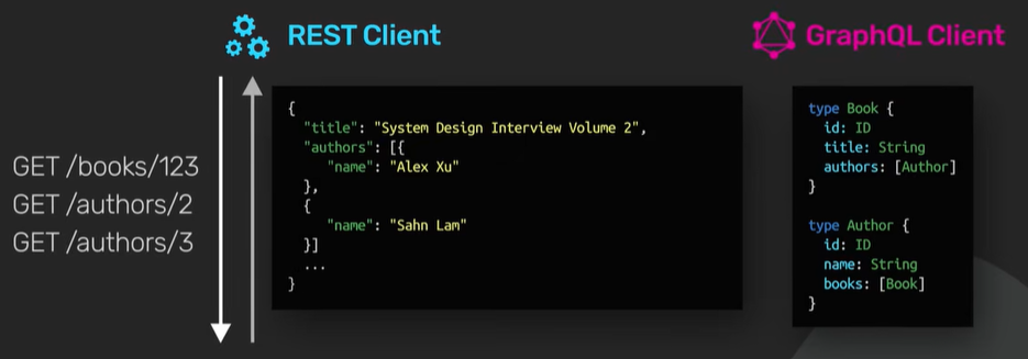
The types describe the kinds of data available. They don’t specify how the data is retrieved via GraphQL.
To do that we need to define a query type Query{ book(id: ID!): Book }
Now we can send a request to the graph ql endpoints to fetch the same data as we can see rest in graph ql both use http both make a request via a url and both can return adjacent response in the same shape.
REST - GET /books/123 and GraphQL - GET /graphql?query={book(id="123"){title,authors{name}}}
Specify the exact resource book and the field like the title and authors.
In REST the api decided author will be inside a resource. In GraphQL user decide what to include in the response.
GraphQL does not use the URL and it uses the schema.
Rest the work in the client side and say first get the books then the author details and it is a N+1 problem.
Drawback - REST does not need any libraries to consume someone else API. Request can be send using common tools like curl or browser. GraphQL requires heavier tooling support both on the client and server size.
GraphQL + Apollo - schema.geaphql, codegen.yaml, operation.graphql
It is more difficult to cache REST users http get for fetching resources and http get has a well defined caching behaviour that is leveraged by browsers, cdns, proxies and web servers. GraphQL has a single point of entry and uses http post by default this prevents the full use of http caching. With care GraphQL could be configured to better leverage http caching the detail is very nuanced.
While GraphQL allows client to query for just the data they need this also poses a great danger. Example where mobile applications shipped a new feature that causes an unexpected table scan of a critical database table of a backend service. This could bring the database down as soon as the new application goes live. It can be solved but it is complex. It should be monitored before choosing GraphQL.
What is Single Sign On.
SSO is an authentication scheme enables a user to securely access multiple applications and services using a single id.
Integrated into apps like Gmail, Workday or slack it provides a pop up widget or lock in page for the same set of credentials with SSO user can access many apps without having a lock in each time.
SSO is built on a concept called Federated identity.
It enables sharing of identity information across trusted but independent systems.
There are two common protocols for this authentication process - SAML and OpenID.
SAML or Security Assertion Markup Language is an xml based open standard for exchanging identity information between services. It is company found in the work environment.
OpenID connect we use when sign in to Google a box appear. It uses JWT to share identity information between services.
How SSO works.
Using protocol SAML, An office worker visits an application like Gmail in SAML terms Gmail in this example is a service provider.
The Gmail Server detects that the user is from the work domain and returns a SAML authentication request back to the browser.
The browser redirects the user to the identity provider for the company specifying the authentication request okta all zero and one logging are subcommon examples of commercial identity providers the identity provider shows the market page where the user enters the log in the passions once the usage is authenticated the identity provided generates a sample response and returns that to the browser this is called a sample assertion the sample assertion is a cryptographically signed xml document that contains information about the user and what the user can access with the service provider the browser forwards the science and constitution to the service provider now the service provider validate that the assertion was signed by the identity provider this validation is usually done with public key cryptography the service provider returns the protective resource to the browser based on what the user is allowed to access as specified in the sample assertion.
SSO integrated application say work day to work day server as in the previous example with Gmail it has to work domain and sends a sample authentication request back to the browser now the browser again we direct the user to the identity provider the user has already logged in with the identity provider it skips the lock in process and instead generates a sample assertion for work day detailing what the users can access there the sample assertion is returned to the browser and forwarded to Woody woody validates the sign assertion and grants user access accordingly the earlier we mentioned that open ID connect is another common protocol the open ID connect flow is similar to Sam but instead of passing sign excel documents around open id connect passes jwt jwt is assigned Json Docket the implementation details are a little bit different but the overall concept is to say so which one of these ssl methods should we use both implementation are secure for an enterprise environment where it is common to outsource identity management to a commercial identity platform the good news is that many of these platforms provide strong support for both so the decision that depends on the application being integrated and which protocol is easier to integrate with if we are writing a new web application integrating with some of the more popular open id connect platforms like Google Facebook we’ll get them is probably a safe bet.
What is a CDN.
https://youtu.be/RI9np1LWzqw?si=usMw70pdgM0y3mSH
Why should we developers all take advantage of it? Let’s take a look. CDN, or content delivery network, has been around since the late 90s. It was originally developed to speed up the delivery of static HTML content for users all around the world. CDN has evolved over the ensuing decades. Nowadays, a CDN should be used whenever HTTP traffic is served. What can a modern CDN do for us? Let’s take a closer look. At a fundamental level, a CDN brings content closer to the user. This improves the performance of a web service as perceived by the user. It is well-documented that performance is critical to user engagement and retention. To bring service closer to the users, CDN deploys servers at hundreds of locations all over the world. These server locations are called Point of Presence, or PoPs. A server inside the PoP is now commonly called an edge server. Having many PoPs all over the world ensures that every user can reach a fast-edge server close to them. Different CDNs use different technologies to direct a user’s request to the closest PoP. Two common ones are DNS-based routing and Anycast. With DNS-based routing, each PoP has its own IP address. When the user looks up the IP address for the CDN, DNS returns the IP address of the PoP closest to them. With Anycast, all PoPs share the same IP address. When a request comes into the Anycast network for that IP address, the network sends the request to the PoP that is closest to the requester. Each edge server acts as a reverse proxy with a huge content cache. We talked about reverse proxy in an earlier video. Check out the description if you would like to learn more. Static contents are cached on the edge server in this content cache. If a piece of content is in the cache, it could be quickly returned to the user. Since the edge server only asks for a copy of the static content from the origin server if it is not in its cache, this greatly reduces the load and bandwidth requirements of the origin server cluster. A modern CDN could also transform static content into more optimized formats. For example, it could minify Javascript bundles on the fly, or transform an image file from an old format to a modern one like WebP or AVIF. The edge server also serves a very important role in the modern HTTP stack. All TLS connections terminate at the edge server. TLS handshakes are expensive. The commonly used TLS versions like TLS 1.2 take several network round trips to establish. By terminating the TLS connection at the edge, it significantly reduces the latency for the user to establish an encrypted TCP connection. This is one reason why many modern applications send even dynamic uncacheable HTTP content over the CDN. Besides performance, a modern CDN brings two other major benefits. First is security. All modern CDNs have huge network capacity at the edge. This is the key to providing effective DDoS protection against large-scale attacks - by having a network with a capacity much larger than the attackers. This is especially effective with a CDN built on an Anycast network. It allows the CDN to diffuse the attack traffic over a huge number of servers. Second, a modern CDN improves availability. A CDN by its very nature is highly distributed. By having copies of contents available in many PoPs, a CDN can withstand many more hardware failures than the origin servers. A modern CDN provides many benefits. If we are serving HTTP traffic, we should be using a CDN. If you would like to learn more about system design,
What is RPC.
GRPC is an open source remote procedure called framework created by Google in 2016. It was a rewrite of their internal rpc infrastructure that they used for years.
What is an RPC or a Remote Procedure Call?
A local procedure call is a function call within a process to execute some code a remote procedure called enables one machine to invoke some code on another machine as if it is local function call from a user’s perspective.
A GRPC is a popular implementation of RPC many organisations have adopted GRPC as a preferred RPC mechanism to connect a large number of microservices running within and across data centres.
GRPC has a thriving developer ecosystem it makes it very easy to develop production quality and type saving apis that scale well the core of this ecosystem is to use a protocol buffers as its data interchange format.
Protocol buffers is a language agnostic that platform agnostic mechanism for encoding structured data gfc uses protocol buffers to encode and send data over the wires by default while GRPC could support other encoding formats like Json protocol buffers provide several advantages that makes it the encoding format of choice for GRPC protocol buffer support strongly typed schema definition the structure of the data over the wire is defined in a prototype protocol buffers provide broad tooling support to turn their schema defying the portal file into data access classes for all popular programming languages a gopc service is also defined in a profile by specifying all pc method parameters and return types the same tooling is used to generate grpc client and server code from the profile developers use these generator classes in the client to make rpc calls and in the server to fulfil the rpc request by supporting many programming languages the client and server can independent No he choose the programming language and ecosystem best suited for their own particular use cases this is traditionally not the case for most other C frameworks the second reason why GRPC is so popular is because it is high performance out of the box 2 factors contributes to his performance first is the protocol buffer is very efficient binary encoding format it is much faster than Jason 2nd GMPC is built on top of HGTP 2 to provide a high performance foundation at scale the use of HTTP2 brings many benefits we discussed HTTP2 in an earlier video cheque out the link in the description for more information gfc uses http 2 streams it allows multiple streams of messages over a single long leaf tcp connexion this allows the GRPC framework to handle many concurrent RPC calls over a small number of tcp connexions between clients and servers to understand how.
Very small number of TCP connexions between clients and servers to understand how GRPC works let’s walk through a typical flow from AGRPC client to AGRPC server in this example the order service is the grpc client and the payment service is the grpc server when order service makes a gopc call to the payment service it invokes the client code generated by GRPC tooling at build time it’s generating client code is called a client stop GOPC encodes the data pass to the client’s step in the protocol buffers and sends it to the low level transport layer share PC sends the data over the network as a stream of HTTP2 data freaks because of Binary Encoding and network optimization gfpc is said to be five times faster than Jason the payment service receives the packets from the network decodes them and invokes the server application the result return from the server application gets encoded into protocol buffers and sent to the transport layer the order service receives the packets decoder and sends the result to the client application as we see from the example above GRPC is very easy to implement it is so easy why do we not see widespread use of GRPC between web clients and web servers one reason is that gopc relies on lower level access to HTTP2 primitives no browsers currently provide the level of control require over web requests to support AGRPC client it is possible to make GRPC calls from the browser with the help of a proxy this technology is called GRPC Web however the feature set is not fully compatible with GRPC and its usage remains low compared to GLPC itself so where does G L P C shine UGRPC and his usage remains low compared to GRPC itself so where does GRPC shine and when should we use it GRPC is the inner service communication mechanism of choice between micro services in the data centres his broad support for many programming languages allows services to choose their own languages and developer ecosystems best suited for their own users we also see increasing use of GRPC in the native mobile clients his efficiency and performance makes a lot of sense in the energy and bandwidth constraint involvements that are mobile devices.
SSL, TLS, HTTPS.
What is so important about these days most websites require it how does https work will answer this question in this video let’s type right in without https the communication between the browser and the server is in plain text this means that the password you enter or the credit card number you sent over Internet can be read by anyone who has the ability to intercept it https is designed to solve this problem to make the data sent over Internet unreadable by anyone other than the sender and the receiver https is an extension of the http protocol we discussed http in an earlier video cheque the description you would like to learn more about we’ve https data is sending an encrypted form using something called tls tls stands for transport layer security if the encrypted data gets intercepted by a hacker all they can see is jumbo data let’s take a look at how the tls can shape works there are several steps step one just like in the case for http the browser establishes a tcp connexion with the server step 2 this is where the tls handshake begins the process sends a client hollow to the server in this hello message the browser tells the server the following things one what tls version it can support it could be tls 1.2 tls 1.3 etc 2 what cyber suites it supports the cyber suite is a set of encryption algorithms to use encrypt data after receiving the client hello the server gets to choose the server suite and the tails version to use based on the options it got from the client it sends those in the server halo message back to the client the server then sends the certificate to the client the certificate includes a lot of different things one of the key things is the public key for the server the client uses the public key in something called asymmetric encryption in a symmetric encryption a piece of data is encrypted by public key can only be decrypted by the private key we’ll discuss how this is used in it this concludes that too the halo phase of the TLS handshake at this point the client has a service certificate and the client and server have agreed on the TLS version and the cyber suite to use now the step 3 this is a step where the client and the server come up with a share encryption key to use the encrypted data and this is where the symmetric encryption coming to the picture again with a symmetric encryption the data encrypted on the client side using the public key from the server can only be encrypted by the server this is how the client sends an encryption key safely to the server over the wide open internet all this is done in the client key exchange message the exact detail varies depending on the cyber suite used here we use rsa as an example since it is the easiest to understand with rsa the client generates an encryption key also call a session key encrypts it with the server public key and sends the encrypted session key to a server over the Internet the server receives the encrypted session key and decrypts it with this private key now both sides hold the session key and this is where they enter step 4 of the TLS handshake where they use the session key and agree upon cyber suite to send encrypted data back and forth in a secure bidirectional channel now you may ask why don’t we just use asymmetric encryption for everything why switch to symmetric encryption at all the main reason is that asymmetric encryption is computationally expensive it is not really suitable for bulk data transmission before we close there are two finite points I would like to discuss first the hashing we talked about applied to tls 1.2 while the latest version is tls 1.3 and tls 1.3 is supported on all major browsers as we can see in our illustration TR is 1.2 takes two network graph trips to complete this is one of the major improvements of tls 1.3 it optimises the handshake to reduce the number of network round trips to one we decided to talk about tls 1.2 because we reviewed tls 1.3 as an optimization as with most optimizations it is a bit harder to explain this is why we chose TRS1.2 instead the core concepts in TLS 1.2 still applies to TLS 1.3 the second final point would like to discuss is that in the explanation about we use RSA for asymmetric encryption to securely exchange the asymmetric session key again we chose the rsa because it is easy to understand however asymmetric encryption is not the only way to share the session key between the client and the server in fact the tls 1.3 rsa is no longer supported and it’s the a method for key exchange diffie Hellman is a more common way nowadays for exchanging session keys diffie Hellman is complicated but in a nutshell it uses some advanced math involving large prime numbers to derive a share session key without ever transmitting a public key over the network this is it for https.
Process vs Thread.
A program is an executable file. It contains the code or a set up processor instructions that is stored as a file on disk.
When the code in a program is loaded into memory and executed by the processor it becomes a Process.
An active process also includes the resources the program needs to run. These resources are managed by the operating system. Some examples are processor, register, program counter, stack pointer, memory pages assigned to the process for its heap and stack.
Each process has its own memory address space. One process cannot corrupt the memory space of another process. It means when one process malfunction other processes keeps running.
Chrome takes the importance of the process isolation by running each tab in its own process.
A thread is a unit of execution within a process. A process has at least one thread and called the main thread. Each thread has its own stack. Thread within a process share a memory address space. It is possible to communicate between threads using that shared memory space.
One misbehaving thread can bring down the entire process.
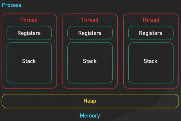
How does the OS run a thread or process on a CPU?
It is handled by context switching.
During a context switch one process is switched out of the cpu so another process can run.
The operating system stores the state of the current running process so the process can be restored and resume execution at a later point. It then restored the previous state of a different process and resumes execution for that process.
Context switching is expansive it involves saving and loading of registers switching out memory pages and updating various kernel data structure.
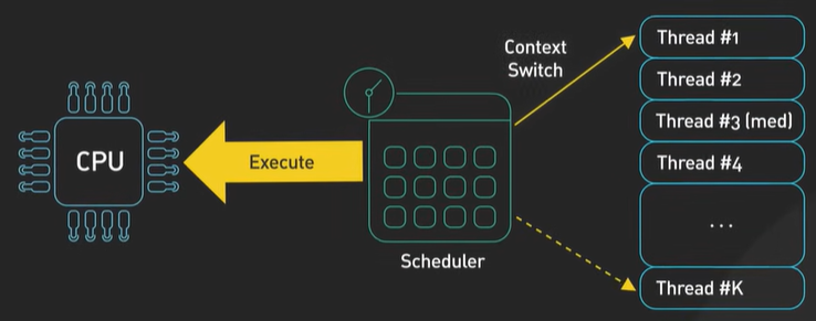
Switching execution between threads requires context switching but it is faster than switching between processes as it shares the same memory so there is no need to switch between virtual memory.
Contact switching is costly and there are other mechanism to minimise it such as fibers and coroutines.
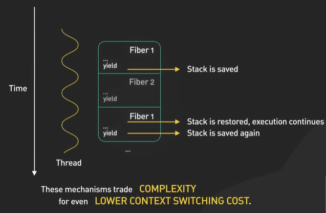
In general they are cooperatively scheduled that is they must yield control for others to run.
In other words the application itself handles task scheduling.
What is OSI Model.
The osi model or the open systems interconnect model is a theoretical framework that provides one way of thinking about networking.
Application Layer.
Presentation Layer.
Session Layer.
Transport Layer.
Network Layer.
Data Link Layer.
Physical Layer.
The physical layer is the bottom most layer it is responsible for transmitting raw bits of data across a physical connection.
The data link layer is the second layer it takes the raw bits from the physical layer and organises them into frames. It ensures that the frames are delivered to the correct destination. The Ethernet primarily lives in this layer.
The network layer is the 3rd layer this is responsible for routing data frames across different networks. The ip part of tcp ip is a well known example of this layer.
The transport layer is the 4th layer it handles end to end communication between 2 nodes this is the layer where tcp and udp live.
TCP provides reliable end to end communication between devices it does this by dividing the data into small manageable segments and sending each segment individually. Each segment has a sequence number attached to it the receiving end uses the secret numbers to reassemble the data in the correct order.
TCP also provides error checking to make sure that the data was not corrupted during transmission udp is another popular protocol in the transport layer it is similar to tcp but it is simpler and faster unlike tcp utp does not provide the same level of error checking or reliability.
It simply sends packets of data from one device to another the receiving end is responsible for determining whether the packets will receive correctly if an error is detected the receiving end simply discards the packet.
The remaining layers are session presentation and application layers this is where the osi model loses its usefulness in practise there are two fine grain and do not really reflect reality. In general this sufficient to collapse them into a single layer and consider application protocols like http and simply layer 7 protocols.
An example to examine how data moves through the layers when transmitting over the network.
When a user sends a http request to a Web server over the network the http header is added to the data at the application layer then the tcp header is added to the data.
It is encapsulated into tcp segments at the transport layer.
The header contains the source port destination port and sequence number.
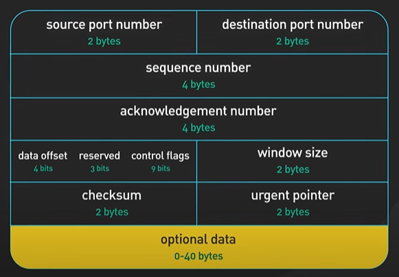
The segments are then encapsulated with an ip header and the network layer.
The ip header contains the source and destination ip addresses a Mac header is added to the data link layer with the source and destination mac addresses.
It is worth noting that in the real world this is a bit nuanced the Mac addresses are usually not the Mac address of the sending and the receiving ends the Mac addresses of the routing devices in the next hop of a usually long journey across the Internet.
The encapsulated frames are sent over the network in raw bits in the physical layer when the Web Server receives the raw bits from the network it reverses the process the headers are removed layer by layer eventually the web server processes the http request.
They are still widely used by networking vendors and cloud providers as a shorthand to describe where the networking products sit in the osi model for example cloud load balances are broadly divided into two categories L4 and L7.
L7 load balancer is a shorthand to mean that the load balancer operates at the application protocol layer like http or https.
L4 load balancer on the other hand operates at the tcp level.
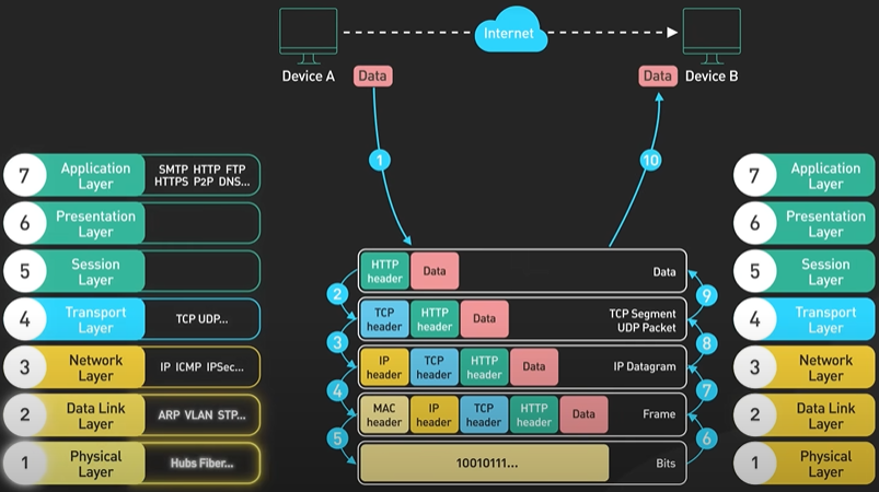
CAP Theorem.
https://youtu.be/BHqjEjzAicA?si=WaJqJOx6YmCBzL5N
What is the CAP theorem? How useful is it to system design? Let’s take a look. The CAP theorem is a concept in computer science that explains the trade-offs between consistency, availability, and partition tolerance in distributed systems. Consistency refers to the property of a system where all nodes have a consistent view of the data. It means all clients see the same data at the same time no matter which node they connect to. Availability refers to the ability of a system to respond to requests from users at all times. Partition tolerance refers to the ability of a system to continue operating even if there is a network partition. But what is a network partition? A network partition happens when nodes in a distributed system are unable to communicate with each other due to network failures. When there is a network partition, a system must choose between consistency and availability. If the system prioritizes consistency, it may become unavailable until the partition is resolved. If the system prioritizes availability, it may allow updates to the data. This could result in data inconsistencies until the partition is resolved. Let’s go through a concrete example. Let’s say we have a tiny bank with two ATMs connected over a network. The ATMs support three operations: deposit, withdraw, and check balance. No matter what happens, the balance should never go below zero. There is no central database to keep the account balance. It is stored on both ATMs. When a customer uses an ATM, the balance is updated on both ATMs over the network. This ensures that the ATMs have a consistent view of the account balance. If there is a network partition and the ATMs are unable to communicate with each other, the system must choose between consistency and availability. If the bank prioritizes consistency, the ATM may refuse to process deposits or withdrawals until the partition is resolved. This ensures that the balance remains consistent, but the system is unavailable to customers. If the bank prioritizes availability, the ATM may allow deposits and withdrawals to occur, but the balance may become inconsistent until the partition is resolved. This allows the system to remain available to users, but at the cost of data consistency. The preference for availability could be costly to the bank. When there is a network partition, the customer could withdraw the entire balance from both ATMs. When the network comes back online, the inconsistency is resolved and now the balance is negative. That is not good. Let’s go through another example and see how a social media platform could apply the CAP theorem. During a network partition, if two users are commenting on the same post at the same time, one user’s comment may not be visible to the other user until the partition is resolved. Alternatively, if the platform prioritizes consistency, the commenting feature may be unavailable to users until the partition is resolved. For a social network, it is often acceptable to prioritize availability at the cost of users seeing slightly different views some of the time. The CAP theorem may sound very simple, but the real world is messy. As with many things in software engineering, it is all about tradeoffs, and the choices are not always so black and white. The CAP theorem assumes 100% availability or 100% consistency. In the real world, there are degrees of consistency and availability that distributed system designers must carefully consider. This is where the simplistic model of the CAP theorem could be misleading. Back to the bank example, during a network partition, the ATM could allow only balance inquiries to be processed, while deposits or withdrawals are blocked. Alternatively, the bank could implement a hybrid approach. For example, the ATM could allow balance inquiries and small withdrawals to be processed during a partition, but block large withdrawals or deposits until the partition is resolved. It is worth noting that in the real world, reconciliation after a network partition could get very messy. The bank example above is simple to reconcile. In real life, the data structures involved could be complex and challenging to reconcile. A good example of a complex data structure is Google Docs. Resolving conflicting updates could be tricky. So is the CAP theorem useful? Yes, it is a useful tool to help us think through the high-level trade-offs to consider when there is a network partition. This is a good starting point, but it does not provide a complete picture of the trade-offs to consider when designing a well-rounded distributed system. Specifically, when the system is operating normally without any network failure, which is most of the time, there is an entire set of interesting trade-offs to consider between latency and consistency. This is covered by the PACELC theorem, which we should cover in another video. If you’d like to learn more about system design, check out our book and weekly newsletter.
Kubernetes.
Kubernetes is an open-source container orchestration platform. It automates the deployment, scaling, and management of containerized applications.
Kubernetes can be traced back to Google’s internal container orchestration system Borg, which managed the deployment of thousands of applications within Google.
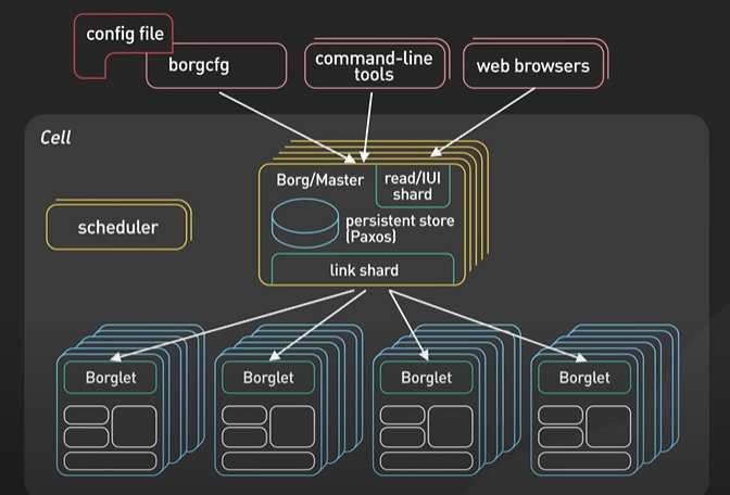
A Kubernetes cluster is a set of machines, called nodes, that are used to run containerized applications.
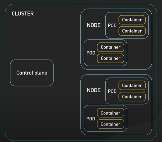
There are two core pieces in a Kubernetes cluster - Control Plane and set of Worker Nodes.
Control plane. It is responsible for managing the state of the cluster. In production environments, the control plane usually runs on multiple nodes that span across several data center zones.
The second is a set of worker nodes. These nodes run the containerized application workloads.
The containerized applications run in a Pod. Pods are the smallest deployable units in Kubernetes. A pod hosts one or more containers and provides shared storage and networking for those containers.
Pods are created and managed by the Kubernetes control plane. They are the basic building blocks of Kubernetes applications.
Control plane. It consists of a number of core components. They are the API server, etcd, scheduler, and the controller manager.
The API server is the primary interface between the control plane and the rest of the cluster. It exposes a RESTful API that allows clients to interact with the control plane and submit requests to manage the cluster.
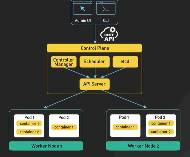
It is used by the API server and other components of the control plane to store and retrieve information about the cluster.
The scheduler is responsible for scheduling pods onto the worker nodes in the cluster. It uses information about the resources required by the pods and the available resources on the worker nodes to make placement decisions.
The controller manager is responsible for running controllers that manage the state of the cluster.
Some examples include the replication controller, which ensures that the desired number of replicas of a pod are running.
apiVersion: v1
kind: ReplicationController
metadata:
 name: nginx
spec:
 replicas: 4
The deployment controller, which manages the rolling update and rollback of deployments. The worker nodes - Core components of Kubernetes that run on the worker nodes include kubelet, container runtime, and kube proxy.
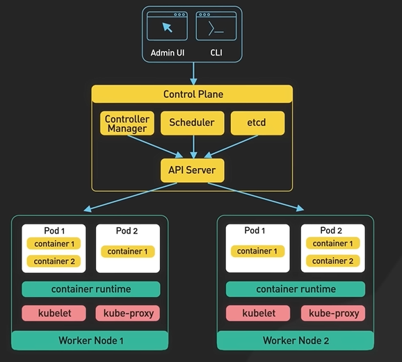
The kubelet is a daemon that runs on each worker node. It is responsible for communicating with the control plane. It receives instructions from the control plane about which pods to run on the node, and ensures that the desired state of the pods is maintained.
The container runtime runs the containers on the worker nodes. It is responsible for pulling the container images from a registry, starting and stopping the containers, and managing the containers’ resources.
The kube-proxy is a network proxy that runs on each worker node. It is responsible for routing traffic to the correct pods. It also provides load balancing for the pods and ensures that traffic is distributed evenly across the pods.
Kubernetes is scalable and highly available. It provides features like self-healing, automatic rollbacks, and horizontal scaling. It makes it easy to scale our applications up and down as needed, allowing us to respond to changes in demand quickly. Kubernetes is portable. It helps us deploy and manage applications in a consistent and reliable way regardless of the underlying infrastructure. It runs on-premise, in a public cloud, or in a hybrid environment. It provides a uniform way to package, deploy, and manage applications.
The number one drawback is complexity. Kubernetes is complex to set up and operate. The upfront cost is high, especially for organizations new to container orchestration. It requires a high level of expertise and resources to set up and manage a production Kubernetes environment.
The second drawback is cost. Kubernetes requires a certain minimum level of resources to run in order to support all the features we mentioned above. It is likely an overkill for many smaller organizations.
One popular option that strikes a reasonable balance is to offload the management of the control plane to a managed Kubernetes service. Managed Kubernetes services are provided by cloud providers.
Some popular ones are Amazon EKS, GKE on Google Cloud, and AKS on Azure.
These services allow organizations to run the Kubernetes applications without having to worry about the underlying infrastructure.
They take care of tasks that require deep expertise, like setting up and configuring the control plane, scaling the cluster, and providing ongoing maintenance and support. This is a reasonable option for a mid-size organization to test out Kubernetes.
For a small organization, YAGNI - You ain’t gonna need it - is our recommendation.
CI CD.
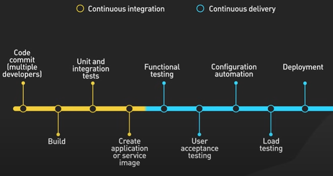
The CICD takes care of the building, testing and deploying the code.
CI - It is a practice to enable automation to enable team to merge code changes into the shared repository. Each commit triggers an automated workflow in a CI server and runs a series of task to make sure the commit is safe to merge.
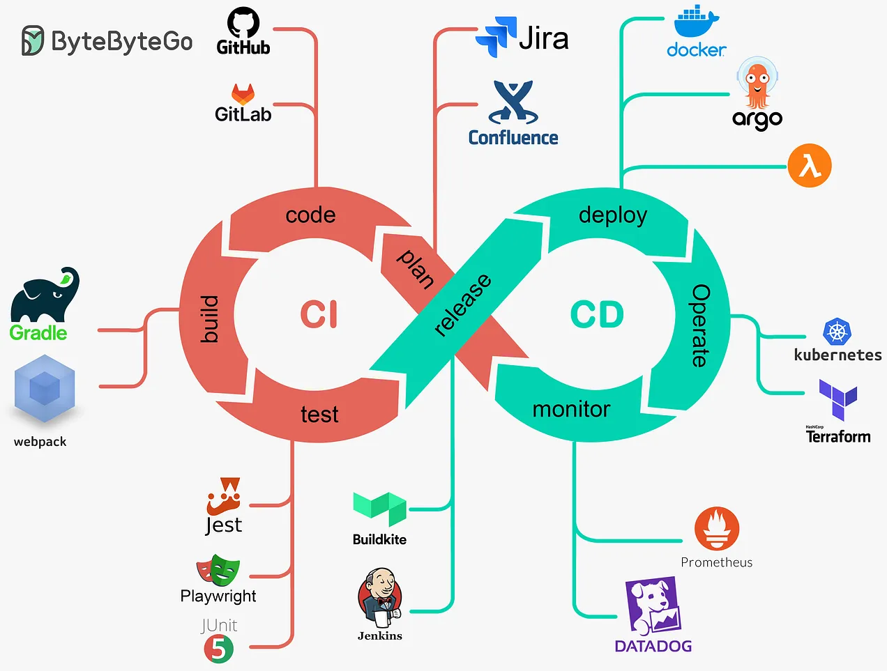
CD - Github Action, BuildKite and Jenkins are commonly used to handle the CD tasks.
There are infrastructure specific tools that will make the CD easier like the ArgoCD in Kubernetes.
https://blog.bytebytego.com/p/a-crash-course-in-cicd
Data Structure that power Modern Database.
All possible test I write in first step is skip list the skip list is a probabilistic data structure that is used to implement a sort of set it is an alternative to a balance tree this allows for efficient search insertion and deletion operations in an in memory database like Reds a skip message used to implement the order data structure such as sort of set it allows a fast look up range queries and other operations next is hash index the hash index also known as a hash table is used to efficiently map keys to values by using a hash function to generate a hash value for each key the hash value is used to quickly locate the value in the table allowing for fast lookups insertions and Deletions hash index is ubiquitous this obviously is used to implement hash data structures by hashes in redis but it’s also widely used internally in all kinds of databases the next two data structures go hand in hand their ss table and lsm tree ss table or soda strain table is used to store data on disc in a sorted order it is a file based data structure that is used to store large amounts of data in a highly compressed and efficient format as a table is a core component of the lsm tree the other core component is a map table mem Table is an in memory data structure that stores recent rights that’s a stable and mem table work together to handle a high volume right operations we have an entire video dedicated to the lsm tree cheque out the description below for a link to the video lsm tree is the backbone of popular nosql databases such as Apache Cassandra Rocksdb and level db next up is the B tree family we include AB plus tree in this the B tree family of data structures are used to efficiently store and retrieve large events of data on disc petri is a balanced tree where each node can have multiple children and keeps data sorted people’s tree is a specific type of B tree where all data is stored in leaf nodes and internal not only whole keys they are widely used in databases such as Mysql Postgres and Oracle to handle large amounts of on this data next is inverted index and inverted index is usually efficiently searched and retrieved data from a large collection of text documents it creates a mapping of words to documents in which they appear the index is inverted because it maps the words to the documents rather than the other way around in order to indexes the company used in document search engines by elastic search next is suffix tree it is used in databases for efficient text searching it quickly finds all occurrences of a search term within a large collection of documents the last data structure we will discuss is somewhat specialised it is artery and artery is a special index data structure that organises data based on their geometric boundaries such as rectangles or polygons it is used to efficiently store and retrieve spatial data in a database it allows for fast spatial queries and is widely used in spatial databases that post gis mongo db and elasticsearch.
System Design Interview.
The 4 steps of a framework - Step two proposed high level design and get by in step 3 design deep dive and step 4 is weather this framework works well for a typical 45 to 16 minutes long system design interview session initially the first five minutes is an introduction and the last slide is Q and A to meet up the interview is only about 35 to 45 minutes we suggest allocating about five minutes to step 120 minutes to step 215 minutes to step three and five minutes to step four now keep in mind this is just a rough guideline feel free to adjust as needed let’s take a closer look at each of the 4 steps set 1 understand the problem and establish design scope system design questions are usually open ended sometimes they are presented in a way that is deliberately vague this test our ability to organise our thoughts and focus on what is important it’s our job to ask as many questions as necessary to understand the problem fully it’s a red flag to jump right into a solution without 1st understanding what we’re building what questions we ask a goal is to clarify the requirements we want to understand why we are building a system who the users are and what features we need to build for example we are asked to design in China it is important to recognise that there are many different types of chatter in the marketplace they are 1 on 1 and small group chat apps like Whatsapp office chat apps like slag or group chat apps like this one they have different design challenges and constraints the goal is to understand the features we are building in priority order we should focus on the top few features to build make sure the interviewer agrees to the feature list it’s also important to ask questions to clarify the non functional requires for system design interviews we suggest focusing on scale and performance these are functional requirements what make a design unique and challenging for example designing a Twitter clone to support a few hundred users is easy while designing it for hundreds of millions of users with some popular accounts having millions of followers is interesting and challenging but the more senior the world is the more important it is for us to demonstrate our ability to handle the non functional requirements but help us get a sense of the scale of the system and the potential challenges and bottlenecks we might do some run back of the inflow calculations here keep in mind that I’m in the potential challenge so the map we do here is a rough estimate the goal is to get a general sense of the scale we want to get the order of the magnitude right but this step should take about 5 minutes at the end we should have a shortlist of features to design for along with the few important non functional requirements to satisfy for sample of a framework we aim to develop a high level design and regional agreement with the interviewer on the design for most designs we will suggest a top down approach and start with the Apis the Apis establish a contract between the end users and the backend systems they should be clear after gathering the requirements what Apis would need unless it is specified otherwise we should follow the restful convention define each api’s input parameters and output responses carefully take the time to carefully review the apis verify that they satisfy the functional requirements equally important to remember do not introduce apis that have nothing to do with the functional requirements an additional consideration on api some designs we call for two way communication between client and server but in this scenario websocket is a common solution here two way communication between client and server and in this scenario websocket is a common solution here be mindful that a socket service websocket is usually stay full it’s quite challenging to operate a scale the scale is high be prepared to discuss how we would manage the websocket deployment in the deep dive section once we have established apis between the client and the server the next step is to layout the high level design diagram the diagram is a blueprint of the overall design that we can refer back to we should use it to verify that the design satisfies all the feature requirements end to end for many designs we start with a load balancer or an api gateway behind that other services that will satisfy the feature requirements we established earlier with the interview many services require some form of persistence this is where we would run out the design by introducing a data storage layer it’s usually not necessary to specify the exact database technology to use at this stage this should be deferred to the deep side section if necessary and only after we have designed the data schema for example for a map service that Google Maps the client often needs to send frequent gps updates to the server we include a designer location data store that a location update service would write to repeat the steps above and complete the high level design diagram for all the major features here’s a project while developing the high level design maintaining a list of discussion points for later resist the temptations to take into too much detail too early do not take a self into a hole before we have a full picture of the design the last step with the high level design is to hash out the data modelling schema here we should discuss the data access patterns and the read write ratio and scale data modelling can significantly impact the performance of the design it is simple also discuss the databases to choose and maybe discuss the indexing options here we should make some judgement calls if the data modelling is the key part of the design to satisfy the non functional requirements we might want to defer the discussion to the deep dive section but we are done with the high level design take a step back and review the design make sure each feature is complete end to end here we reach the 3rd step of the framework design deep dive the goal of this section is to demonstrate that we could identify areas that could potentially be problematic and come up with solutions and discuss trade offs we should work with the interview closely to decide what to discuss in the data is wearing on functional requirements make the problem interesting the higher the level the more important this section is the section is really open ended there is no one size fits all approach Who made the world’s useful sometimes again who was body language we give away clues that they are dissatisfied with certain aspect of the design this is important to pick up these clues and make sure the issues are addressed one way we can approach it is by asking questions we can list out the reasons for choosing a particular solution and ask if they have any questions or concerns once we pick out a problem or two to dive deeper into we should cover with multiple solutions and discuss trade offs for each option we can use the following meaning guidelines when framing the discussions first we should clearly articulate a problem for example for designing Google Maps the right qps at 1 million per second to the location database is too high for single database to end next we come up with at least two solutions continuing with example above we could propose to reduce the location update frequency per user or choose a number sql database that could handle the right rate 3rd we discussed the trade offs of the solutions remember to use numbers to back up our design finally we pick a solution and discuss it with the interview now repeat this for other problems in a typical interview we should only have time to dive deeper into the top 2 or 3 issues lastly we have reached the last step wrap up we suggest spending a few minutes summarising the design here we should focus on the parts that are unique to the particular situation keep it short and sweet leave enough room at the end of the interview to ask the interviewer questions about the company that’s it on the system design interview framework we hope you find it useful
Top 5 Redis use case.
In this video we discovered a versatility of wealth we talked about the top use cases they have metal testing in production the various companies and the various scales interesting scalability challenges for us hello why is a great tool to know well in our system design tool set let’s type right to it first of all what is rabbits and why do people use it president in memory data structure store is most commonly used as a cache it puts many data structures such as strings caches lists sets and soda sets redis is known for speed we made a video to explain why redis is so fast look for the link in the description we would like to watch that video let’s dive into the top use cases of Redis the number one use case in Redis is cashing objects to speed up web applications in this case Redis source frequently requested data in memory it allows the web servers to return frequently access data quickly this reduces the low on the database and improves the response time for the application a scale the cache is distributed among the cluster of red servers shotting is a common technique to distribute the caching load even across the cluster other topics you consider when deploying redis as a distributed cache include setting a correct ttl and handling thundering hurt or costar another common use case is to use radis as a session store to share session data about servers when I use the logs into a web application the session data is storing redis along with a unique session id that is returned to the client as a cookie when the user makes a request to the application the session id is included in the request and the status web server retrieves the session data from Redis using the id at least important note the redis is an in memory database the session data stored redis will be lost if the Reddit servers restarts even though Redis provides persistent options by a snapshot at AOF will depend only file the last session data will be saved to disc and reloading the memory in the event of a restart these options often take too long to load to be practical in production replication is usually used instead in this case data is replicated to a backup instance in the event of a crash of the main instance the backup instance is quickly promoted to take over the traffic the next use case is distributed lock distribute the locks are used when multiple nodes in an application need to coordinate access to some shared resource redis is used as a distributor lock with this atomic commands like set annex or set if not exists it allows the caller to set a team only if it is not already exist this is how it works at a high level client one tries to acquire the lock by setting a key with a unique value in a timeout using a set and X Command the key was not already set the set annex command returns one indicating that the lock has been inquired by time 1 time 1 finishes his work and releases the lock by deleting the key but if the key was already set the set annex command returns zero indicating that the lock is already been held by another client in this case client waits and retries a set an X operation until the lock is released by the other client look at this simple implementation might be good enough for many use cases but it’s not completely fault tolerant for protection news there are many redis claimed libraries they provide high quality distributed log implementation right off the box next up is rate limited redis can be used as a rate limiter by using incremental command on some counters and setting exploration times on those counters a very basic rate limiting algorithm works this way for each incoming request the request ip or user id is used as a key the number request for the key is increment using the increment domain the current is compared to the allow rate limit if the count is within the rate limit request is process if the count is over the limit the request is rejected the keys are set to expire after specific time window for example a minute to reset the cans for the next time window most sophisticated rate limiters by the leaky bucket algorithm can also be implemented using Redis the last use case we would like to talk about is gaming leader for most games they are not super high scale redis is a delightful way to implement various types of gaming leaders but a fundamental data structure that enables us a solar set is a collection of unique elements associated with it the elements are sorted by score this allows a quick retrieval of elements by score in logarithmic time.
Debugging.
https://youtu.be/J8uAiZJMfzQ?si=dseWl62OcUtX60AA
Have you ever wondered why debugging is not taught in school? Most developers actually learn it on the job, and only a lucky few have a mentor to guide them through the process. In this video, we’re going to present a systemic approach to debugging that you can use as a checklist on your debugging journey. Debugging demands discipline, and it’s easy to get off course and waste valuable time. We’ll show you how to make sound tradeoffs and use good judgment. So whether you’re a beginner or an experienced developer, this video is for you. Follow along as we share our tips and tricks for effective debugging. And remember, feel free to use these in any order - there’s no right or wrong way to debug! Let’s start by discussing the importance of having the right mindset when it comes to debugging challenging problems. It can mean the difference between giving up too early or ultimately solving the issue. When facing tough debugging challenges, it’s important to keep the following things in mind: First, remember that computers are logical, and there is always a logical explanation for the issue at hand, even if it may seem impossible to find at the moment. Secondly, being stuck is only temporary, and with persistence and effort, the issue will eventually be resolved. Third, it’s important to know your limits and recognize when it’s time to seek help from others who may have more expertise. Lastly, it is not always necessary to spend a significant amount of effort in resolving every bug. We should prioritize bugs based on their potential impact and severity. We should accept that fact that some bugs may not be worth the effort. Let’s start by covering the basics. When we receive a bug report from a customer, it’s important to gather as much information about it as possible. Request a screenshot or screen recording from the customer if possible. Additionally, collect detailed steps to reproduce the issue, and gather all relevant logs, including any error messages associated with the bug. The goal is to obtain as much information as possible to help us reproduce the problem. If we can isolate the environment and context where the issue occurs, we can try to recreate it on a staging server and see if we can reproduce the problem. Having a reproducible environment is half the battle. Now that we have a reproducible environment, how should we investigate the bug? Here are a few strategies to consider: First, use print statements liberally. They can help construct a timeline of what happened and determine if the events we expected to happen in the code actually line up with the print statements. For some language ecosystems, setting up a debugger may be a viable option. For example, systems like Erlang/OTP have excellent introspection capabilities, making the debugger an excellent first tool to reach for. Ultimately, if we can reproduce the bug, it should not be too difficult to get to the bottom of it. While it will take time and patience, following the strategies we mentioned should help us solve the issue eventually. What if we can’t reproduce the issue? Well, that’s much tougher. It may require some luck and a lot of patience. Let’s try to understand why we sometimes have so much trouble reproducing the issue. Here are a few common scenarios: Some bugs only appear under production loads. Some bugs only appear under production loads in certain race conditions. There may be specific context or environment on the customer’s device that triggers the bug. What can we do in these situations? Here are a few ideas: If there is a specific error, retrace the code from the line where the error occurred all the way up the call stack. Comb through all the logs for clues and build a timeline by following one failed request through the entire request lifecycle. If we’re lucky, we may be able to come up with a theory as to what is happening. Next, we can add logging to the code to prove the theory and deploy it to production or ship it to the customer. Repeat this process until we gather more clues and eventually solve the issue. Keep in mind that this cycle can be lengthy and frustrating, but persistence is key. Lastly, let’s review some general strategies to consider when we’re completely stuck: Take a break. Sometimes, stepping away from the problem and coming back with a fresh mind can provide new insights. Sleep on it, get some exercise, or engage in a different activity to clear your mind. Tea drinking, some yoga, field of grass visualization etc. Get a rubber duck. Sometimes, talking about the problem out loud can lead to a “light bulb” moment. For others, writing out the problem or emailing an imaginary mentor can help generate new ideas and perspectives. Get help. Don’t hesitate to collaborate with someone else on the problem. A fresh set of eyes and a different perspective can often help to reveal new solutions. Debugging can be tough, but with the right mindset and strategies, you can overcome any challenge. Good luck. If you like our videos, you may like our weekly system design newsletter as well.
What is Cloud Native.
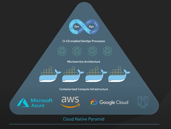
Cloud Native was first introduced by Netflix in 2013 in an AWS event when Netflix discussed the web-scale architecture.
Cloud 90 for the blueprint for designing web scale application on the cloud that are more available and scalable.
It promises agility to ship new features quickly without compromising the availability.
Confusion between cloud native and cloud computing?
Cloud computing is running application on computing resources managed by cloud providers without having to purchase and manage hardware separately.
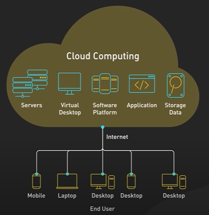
Migrate an application from monolith to on-prem is one way.
Running application to cloud does not make it cloud native. The application to be cloud native should follow 4 pillars.
Microservices, Containers, DevOps, Cloud Native Open Standards.
Application Architecture - Cloud Native architecture is made up of small interdependent microservices.
Containers - Container orchestration - Application are within the containers and it contains everything to run the microservice. When the number of microservice grows the container orchestration helps to manage the containers. Example - Kubernetes - It controls where containers run, Detect and repair and Balance load between microservices.
DevOps - Development and deployment process.
Cloud Native Open Standard - Following the components and standards.
Example of some well known standards and application.
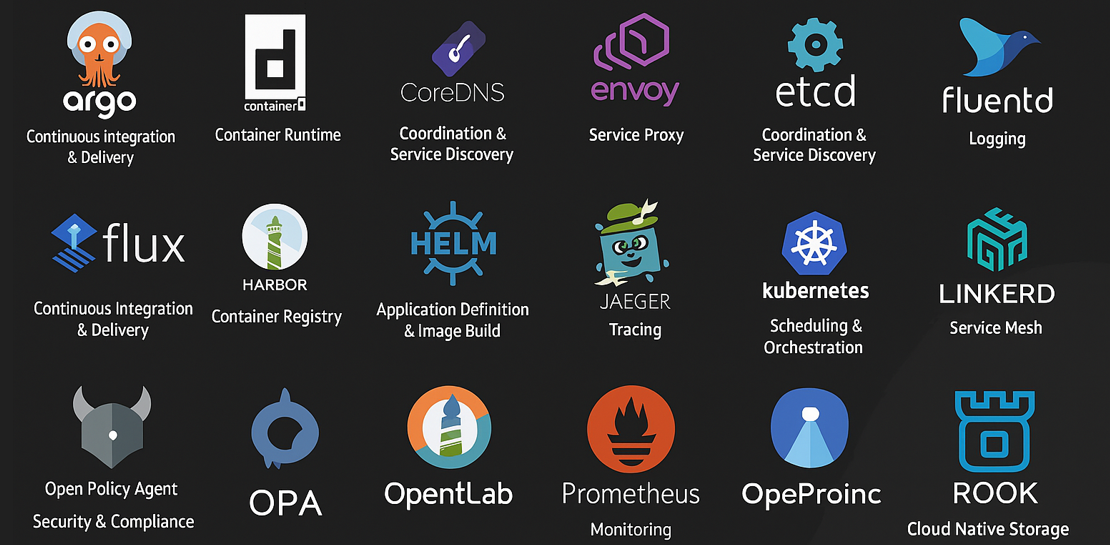
Jaeger, Zipkin, OpenTelemetry.
Service Mesh is a core infrastructure layer for managing service to service communication between microservcies.
Istio and Linkerd are some of the example.
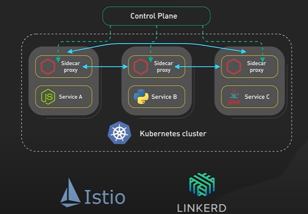
The principle and the standard architecture refers as a cloud native architecture.
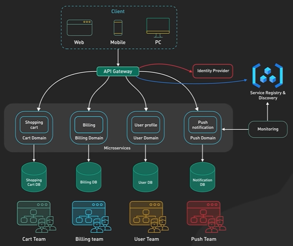
DNS.
DNS, or Domain Name System, is the backbone of the internet. DNS is the internet’s directory. It translates human-readable domain names, such as google.com to machine-readable IP addresses.
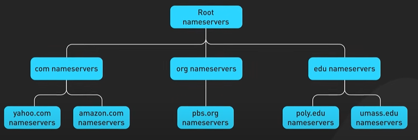
When a browser makes a DNS query, it’s asking a DNS resolver. This DNS resolver could be from our ISP, or from popular DNS providers like Cloudflare’s 1.1.1.1, or Google’s 8.8.8.8.
If the DNS resolver does not have the answer in its cache, it finds the right authoritative nameserver and asks it. The authoritative nameserver is the one that holds the answer.
When we update a domain’s DNS records, we are updating its authoritative nameserver.
How does the DNS resolver find the authoritative name server?
There are three main levels of authoritative DNS servers. They are the Root Name Servers, the Top Level Domain (or TLD) name servers, and the Authoritative Nameservers for the domains.
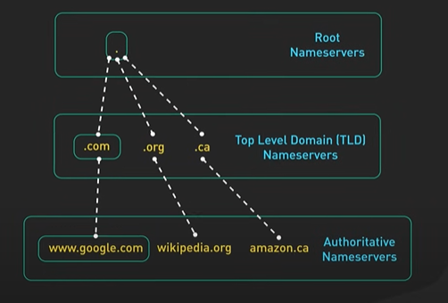
The root name servers store the IP addresses of the TLD name servers.
There are 13 logical root name servers. Each root name server has a single IP address assigned to it. There are actually many physical servers behind each IP address. Through the magic of anycast, we get routed to the one closest to us.
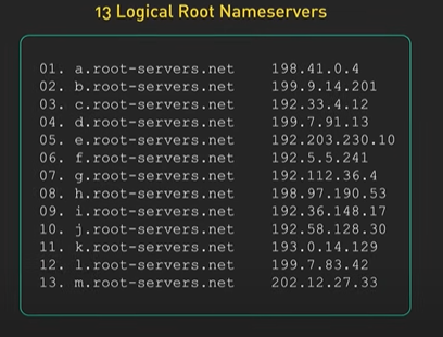
The TLD name servers store the IP addresses of the authoritative name servers for all the domains under them. There are many types of TLD names. We are all familiar with .com, .org and .edu. There are also country code TLDs like .de and .uk.
The authoritative name servers for a domain provide, well, authoritative, answers to DNS queries.
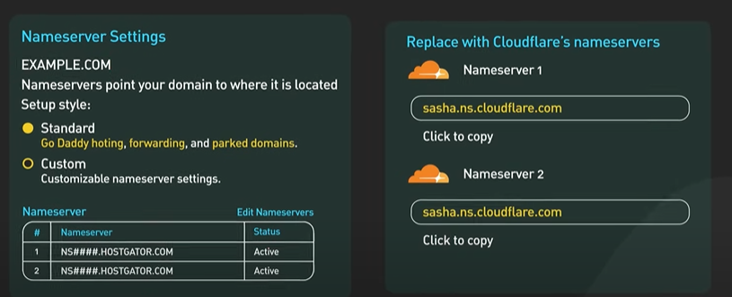
When we register a domain, the registrar runs the authoritative nameservers by default, but we can change them to others. Cloud providers like AWS and Cloudflare run robust authoritative nameservers.
This hierarchical design makes DNS highly decentralized and robust.
The life of a typical DNS query.
The user types google.com into the browser. The browser first checks its cache. If it has no answer, it makes an operating system call to try to get the answer. The operating system call would most likely have its own cache. If the answer isn’t there, it reaches out to the DNS resolver.
The DNS resolver first checks its cache. If it’s not there or if the answer has expired, it asks the root name server. The root name server responds with the list of the .com TLD name servers. Note that since .com is such a common TLD, the resolver most likely already caches the IP addresses for those .com TLD nameservers.
The DNS resolver then reaches out to the .com TLD nameserver, and the .com TLD nameserver returns the authoritative nameservers to google.com.
And finally, the DNS resolver reaches out to google.com’s authoritative nameserver, and it returns the IP address of google.com.
The DNS resolver then returns the IP address to the operating system, the operating system returns it to the browser.
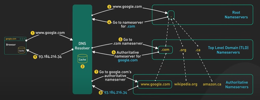
Finally, let’s go over some gotchas when updating DNS records for a live, high-traffic production system.
DNS propagation is slow because there is a TTL on each DNS record. And some of the default TTLs are pretty long. Also, not every DNS resolver is a good citizen. There are some buggy out there that don’t honor the TTL. To mitigate the risk, there are two practical steps to take.
First, reduce the TTL for the record that we want to change to something very short, say 60 seconds, well in advance before the update actually happens. This gives ample time for all the DNS servers to receive the shortened TTL which would allow the actual record update to take effect based on the new shortened TTL.
Second, leave the server running on the old IP address for a while. Only decommission the server when traffic dies down to an acceptable level. Because some DNS resolvers don’t honor the TTL, this could take a bit of time and patience.
Backend Architecture.
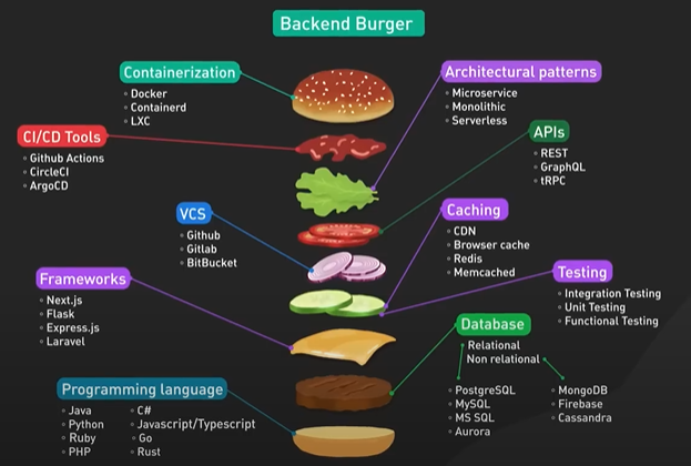
For this particular exercise, we will focus on an early-stage startup, where there are limited resources, and product/market fit is not yet certain. In this scenario, maximum flexibility is preferred.
To maintain maximum flexibility, we will probably go serverless functions.
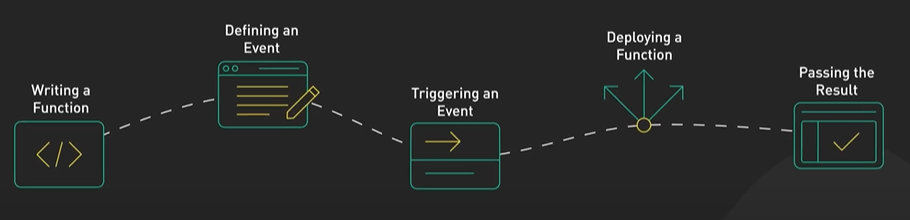
Serverless functions have a very strict request/response programming model, but under the hood, most serverless functions are packaged as a container.
CDN comes for free with most hosting providers like Vercel and Netlify. If not, just use Cloudflare.
If we are storing very simple data, we would use something hosted like Firebase or Firestore. If our data model is more complicated, we would use a serverless relational database like Aurora Serverless.
Types of Memory and Storage.
The fundamental duo: RAM and ROM.
RAM, or Random Access Memory, is a type of memory that stores data temporarily while your computer is running. It’s fast and flexible, juggling all the programs we’re running at any given moment. However, RAM is volatile, meaning it loses its stored data when the power is turned off.
ROM, or Read-Only Memory, is a type of memory that retains data even when the power is off. It’s non-volatile and used to store essential information, like firmware and the BIOS, that your computer needs to boot up.
The different types of RAM, including SRAM, DRAM, and everything in between.
SRAM, or Static Random Access Memory, is a fast and expensive type of RAM used in high-speed applications like CPU caches, where quick access time is crucial.
DRAM, or Dynamic Random Access Memory, is slower and cheaper than SRAM. It needs to be constantly refreshed to retain data, making it more high-maintenance.
There are many types of DRAM, including FPM DRAM, EDO DRAM, SDRAM, and DDR SDRAM many are obsolete.
The common types of DRAM in the market today are DDR4, DDR5.
GDDR is also worth mentioning. It is a specialized type of DRAM optimized for faster data transfer rate, which the GPU needs for its massive parallel processing. GDDR6 is the most widely used today.
Roles of ROM: Firmware and BIOS.
Firmware is a type of software stored in ROM that controls how hardware devices communicate with each other. BIOS, or Basic Input/Output System, is the first software your computer runs when you power it up. It’s responsible for starting your computer, initializing hardware components, and handing control over to the operating system.
Hard Disk Drives, or HDDs, have been around for a long time. They store data on spinning magnetic disks and are known for their large storage capacities at a low price.
Solid State Drives, or SSDs, use NAND-based flash memory, providing faster data access, reduced power consumption, and increased durability compared to HDDs, but come at a higher price.
NVMe, or Non-Volatile Memory Express, is a high-performance interface for SSDs that connects directly to the CPU via PCIe lanes. This allows for lower latency and significantly faster data transfer rates compared to SATA-based SSDs.
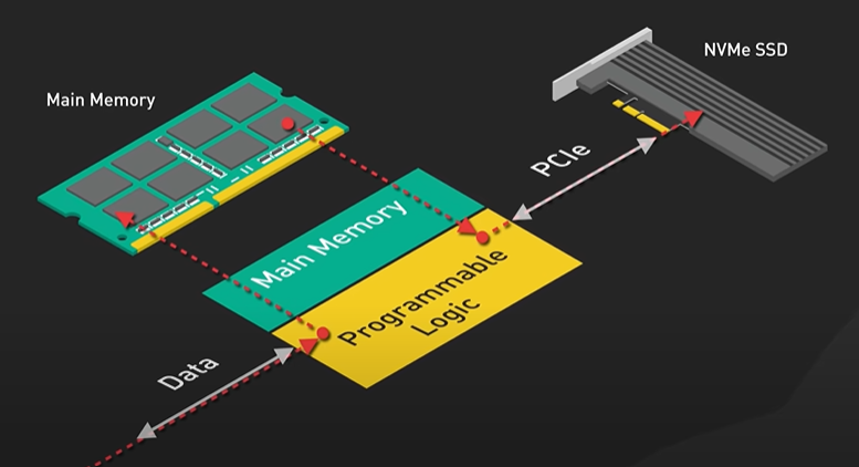
Need to take your data on the go - Flash Drives and SD Cards.
Flash Drives, also known as USB drives or thumb drives, are small, plug-and-play devices you can use with any USB port. They’re easy to use and perfect for transferring files between computers.
SD Cards are commonly found in cameras and smartphones. They’re smaller than a postage stamp but can store thousands of files. SD cards come in three main physical sizes: SD, microSD, and miniSD.
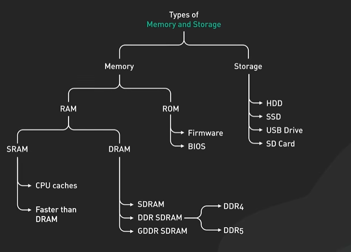
Cache system.
Caching is a technique to enhance system performance and reduce response time.
A typical system architecture involves several layers of caching, depending on the requirements and constraints of the specific application.
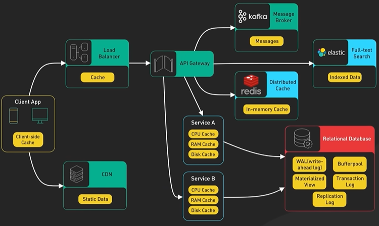
The most common hardware cache are L1, L2, and L3 caches.
L1 cache is the smallest and fastest cache, typically integrated into the CPU itself.
It stores frequently accessed data and instructions, allowing the CPU to quickly access them without having to fetch them from slower memory.
L2 cache is larger but slower than L1 cache, and is typically located on the CPU die or on a separate chip.
L3 cache is even larger and slower than L2 cache, and is often shared between multiple CPU cores.
Another common hardware cache is the Translation Lookaside Buffer (TLB). It stores recently used virtual-to-physical address translations. It is used by the CPU to quickly translate virtual memory addresses to physical memory addresses, reducing the time needed to access data from memory.
At the operating system level, there are page cache and other file system caches.
Page cache is managed by the operating system and resides in main memory. It is used to store recently used disk blocks in memory. When a program requests data from the disk, the operating system can quickly retrieve the data from memory instead of reading it from disk.
There are other caches managed by the operating system, such as the inode cache. These caches are used to speed up file system operations by reducing the number of disk accesses required to access files and directories.
Content Delivery Networks (CDNs) are widely used to improve the delivery of static content, such as images, videos, and other web assets. One of the ways that CDNs speeds up content delivery is through caching.
When a user requests content from a CDN, the CDN network looks for the requested content in its cache. If the content is not already in the cache, the CDN fetches it from the origin server and caches it on its edge servers. When another user requests the same content, the CDN can deliver the content directly from its cache, eliminating the need to fetch it from the origin server again.
Some load balancers can cache resources to reduce the load on back-end servers. When a user requests content from a server behind a load balancer, the load balancer can cache the response and serve it directly to future users who request the same content.
Caching does not always have to be in memory. In the messaging infrastructure, message brokers such as Kafka can cache a massive amount of messages on disk. This allows consumers to retrieve the messages at their own pace. The messages can be cached for a long period of time based on the retention policy.
Distributed caches such as Redis can store key-value pairs in memory, providing high read/write performance compared to traditional databases
Full-text search engines like Elastic Search can index data for document search and log search, providing quick and efficient access to specific data.
Even within the database, there are multiple levels of caching available.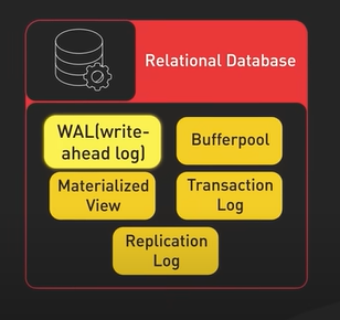
The buffer pool is a memory area used to cache query results, while materialized views can precompute query results for faster performance.
The transaction log records all transactions and updates to the database, while the replication log tracks the replication state in a database cluster.
GPT.
https://youtu.be/bSvTVREwSNw?si=nwd7ew33MXqr1g51
We learned a lot from making this video. We hope you will learn something, too. Let’s dive right in. ChatGPT was released on November 30, 2022. It reached 100M monthly active users in just two months. It took Instagram two and a half years to reach the same milestone. This is the fastest growing app in history. How does ChatGPT work? The heart of ChatGPT is an LLM, or a Large Language Model. The current LLM for ChatGPT is GPT-3.5. ChatGPT could also use the latest GPT-4 model, but there is not much technical detail on GPT-4 for us to talk about yet. What is a Large Language Model? A Large Language Model is a type of neural network-based model that is trained on massive amounts of text data to understand and generate human language. The model uses the training data to learn the statistical patterns and relationships between words in the language, and then utilizes this knowledge to predict the subsequent words, one word at a time. An LLM is often characterized by its size and the number of parameters it contains. The largest model of GPT-3.5 has 175 billion parameters spread across 96 layers in the neural network, making it one of the largest deep learning models ever created. The input and output to the model are organized by token. Tokens are numerical representations of words, or more correctly, parts of the words. Numbers are used for tokens rather than words because they can be processed more efficiently. GPT-3.5 was trained on a large chunk of Internet data. The source dataset contains 500B tokens. Looking at it another way, the model was trained on hundreds of billions of words. The model was trained to predict the next token given a sequence of input tokens. It is able to generate text that is structured in a way that is grammatically correct and semantically similar to the internet data it was trained on. But without proper guidance, the model can also generate outputs that are untruthful, toxic, or reflect harmful sentiments. Even with that severe downside, the model is already useful, but in a very structured way. It could be “taught” to perform natural language tasks using carefully engineered text prompts. This is where the new field “prompt engineering” came from. To make the model safer, and be capable of question and answer in the style of a chatbot, the model is further fine-tuned to become a version that was used in ChatGPT. Fine-tuning is a process that turns the model that does not quite align with human values into a fine-tuned model that ChatGPT could use. This process is called Reinforcement Training from Human Feedback (RLHF). OpenAI explains how they ran RLHF on the model, but it is not easy to understand for non-ML people. Let’s try to understand it with an analogy. Imagine GPT-3.5 as a highly skilled chef who can prepare a wide variety of dishes. Fine-tuning GPT-3.5 with RLHF is like refining this chef’s skills to make their dishes more delicious. Initially, the chef is trained with a large dataset of recipes and cooking techniques. However, sometimes the chef doesn’t know which dish to make for a specific customer request. To help with this, we collect feedback from real people to create a new dataset. The first step is to create a comparison dataset. We ask the chef to prepare multiple dishes for a given request, and then have people rank the dishes based on taste and presentation. This helps the chef understand which dishes are preferred by the customers. The next step is reward modeling. The chef uses this feedback to create a “reward model,” which is like a guide for understanding customer preferences. The higher the reward, the better the dish. Next, we train the model with PPO, or Proximal Policy Optimization. In this analogy, the chef practices making dishes while following the reward model. They use a technique called Proximal Policy Optimization to improve their skills. This is like the chef comparing their current dish with a slightly different version, and learning which one is better according to the reward model. This process is repeated several times, with the chef refining their skills based on updated customer feedback. With each iteration, the chef becomes better at preparing dishes that satisfy customer preferences. To look at it another way, GPT-3.5 is fine-tuned with RLHF by gathering feedback from people, creating a reward model based on their preferences, and then iteratively improving the model’s performance using PPO. This allows GPT-3.5 to generate better responses tailored to specific user requests. Now we understand how the model is trained and fine-tuned, let’s take a look at how the model is used in ChatGPT to answer a prompt. Conceptually, it is as simple as feeding the prompt into the ChatGPT model and returning the output. In reality, it’s a bit more complicated. First, ChatGPT knows the context of the chat conversation. This is done by ChatGPT UI feeding the model the entire past conversation every time a new prompt is entered. This is called conversational prompt injection. This is how ChatGPT appears to be context aware. Second, ChatGPT includes primary prompt engineering. These are pieces of instructions injected before and after the user’s prompt to guide the model for a conversational tone. These prompts are invisible to the user. Third, the prompt is passed to the moderation API to warn or block certain types of unsafe content. The generated result is also likely to be passed to the moderation API before returning to the user. And that wraps up our journey into the fascinating world of ChatGPT. There was a lot of engineering that went into creating the models used by ChatGPT. The technology behind it is constantly evolving, opening doors to new possibilities and reshaping the way we communicate. Tighten the seat belt and enjoy the ride. If you like our videos, you may like our system design newsletter as well.
GPT Developer.
https://youtu.be/9W_U1y7RYuE?si=kXmriyZSZBZcpod7
and if you haven’t jumped on board yet, you’re missing out on a competitive edge. In today’s video, we’ll be giving you a grand tour to ChatGPT, demonstrating how it can supercharge your daily tasks and elevate your efficiency. Don’t get left behind—discover how to harness the power of ChatGPT and stay ahead of the curve in this rapidly evolving world of software development. One of the most common ways software developers use ChatGPT is to get help understanding confusing code. ChatGPT knows a lot about programming languages and can explain how different parts of code work in a simple way. For example, imagine we find this Python code that uses some advanced features like list comprehensions and lambda functions: If we don’t know what’s going on or find the code hard to read, we can ask ChatGPT to explain it. With ChatGPT’s help, we can better understand the code we’re working with and feel more confident when dealing with complex code. Another great way to use ChatGPT is for finding errors and reviewing code. ChatGPT can help us spot mistakes in our code and suggest improvements. When we’re working on a project, it’s common to find that something isn’t working as expected. ChatGPT can look at our code and point out any errors or areas that might need fixing. It can also offer suggestions on how to make our code better. Let’s consider an example in C. We’re trying to implement a function that reverses a null-terminated string in place. Here’s the problematic code: We can ask ChatGPT to help us identify and fix the issue with this code. It tells us that there’s an off-by-one error in the reverse_string function when swapping characters. It even generates the correct code for us! Another useful way to use ChatGPT is to translate code from one programming language to another. This can be really helpful if we get a solution in one language, but our project is in a different language. ChatGPT knows many programming languages, so it can help us make the switch. For example, let’s say we get some Python code that fixes a security issue, but our project is in Rust. We need to change the Python code into Rust, and ChatGPT can help us do that. Here’s an example in Python: We can ask ChatGPT to help us rewrite this code in Rust. The AI might give us this Rust version: With ChatGPT’s help, we can change code from one language to another easily. This saves us time, helps avoid mistakes when doing it by hand, and teaches us more about different programming languages. Another great way to use ChatGPT is to rely on it as we learn a new programming language. A perfect personal example is when we had to complete a project in Rust, which was new to us. We needed to read an object from a Google Cloud Storage bucket in chunks to make it more efficient. So, we asked ChatGPT how to do that. ChatGPT can provide us with guidance, examples, and even code snippets to help us get started with our task. By asking specific questions or for examples, we can learn how to use new libraries, functions, or language features that we’re unfamiliar with. For instance, in this case, ChatGPT might give us an example of how to read an object from a GCS bucket in chunks using Rust. This would include recommendations for libraries and example code that demonstrates how to achieve our goal. By following the guidance provided by ChatGPT, we can quickly gain a better understanding of Rust and complete our project efficiently. By leaning on ChatGPT when learning a new programming language, we can save time and reduce the learning curve, making it easier to adapt to new languages and become proficient in them. Another great way we can use ChatGPT is to write unit tests for our code. Unit tests are important because they help us make sure our code is working correctly and that changes we make don’t break existing functionality. Writing good unit tests can be challenging, and sometimes tedious, but ChatGPT can make it easier for us. Let’s consider a real-world example where we have a TypeScript function that takes a string input and sanitizes it for use in HTML by escaping special characters. Here’s the function: We can ask ChatGPT to help us come up with different test cases to validate the correctness of the sanitizeHtml function. ChatGPT might suggest a few good test cases: And even write the test cases for us: With ChatGPT’s help, we can create comprehensive unit tests for real-world production code, ensuring our code is working correctly and maintaining a high level of software quality. Another great way to use ChatGPT is to modify existing code to add more functionality. With ChatGPT’s understanding of programming languages and software engineering concepts, it can help us enhance our code by suggesting changes or providing new code snippets. Let’s consider a real-world example where we have a TypeScript function that filters out items from an array based on a provided predicate function. Here’s the original function: Suppose we want to modify this function to include an additional feature: an optional parameter that allows us to limit the number of items returned after filtering. We can ask ChatGPT for help in making this change. ChatGPT might suggest adding an optional limit parameter and updating the loop condition to stop once the limit is reached. Here’s the modified function: By using ChatGPT to modify our code and add more functionality, we can save time, ensure that our changes are implemented correctly, and learn new techniques for enhancing our code. Another way we can use ChatGPT is to write documentation and comments for our code. Well-written documentation and comments are crucial for maintaining the readability and maintainability of our codebase. ChatGPT can help us write clear, concise, and informative comments and documentation, even for complex real-world code. Let’s consider a real-world example where we have a TypeScript function that searches for a specified pattern in a given text and returns the indices of all occurrences. Here’s the function: We can ask ChatGPT to help us write comments and documentation for this function, explaining its purpose, parameters, and return value. Here’s what ChatGPT might suggest: By using ChatGPT to write documentation and comments, we can ensure that our code is easy to understand and maintain, making it more accessible to other developers. Here’s a word of caution: It’s important to remember that ChatGPT has its limitations and shouldn’t be relied on blindly. Sometimes it might give suboptimal or flatly wrong answers, so always think critically and ask the right questions. For instance, if we examine the Rust example generated earlier to read an object from a GCS bucket in chunks, we’ll notice that it’s not ideal for very large objects, as it reads the entire object into memory. As software engineers, we are responsible for our code and solutions. Use ChatGPT as a helpful assistant, but make sure to double-check its suggestions and maintain control over your work. ChatGPT is a game-changing tool for software engineers. It helps us tackle complex tasks, understand new languages, and improve our code efficiently. By using ChatGPT, we can become better developers and make our work more enjoyable. Let’s embrace ChatGPT’s potential and see how it revolutionizes the way we code!
Most used System Pattern.
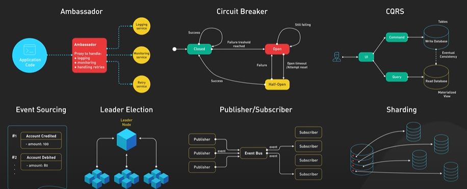
Ambassador pattern acts as a “go-between” for your app and the services it communicates with, offloading tasks like logging, monitoring, or handling retries.
For instance, Kubernetes uses Envoy as an Ambassador to simplify communication between services. The Ambassador pattern can help reduce latency, enhance security, and improve the overall architecture of your distributed systems.
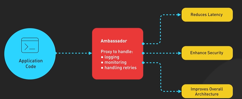
Circuit Breaker - Imagine a water pipe bursting in your house. The first thing you’d do is shut off the main valve to prevent further damage. The Circuit Breaker pattern works similarly, preventing cascading failures in distributed systems.
When a service becomes unavailable, the Circuit Breaker stops requests, allowing it to recover.
Netflix’s Hystrix library uses this pattern. It ensures a more resilient system. This pattern can be particularly useful when dealing with microservices or cloud-based applications, where failures are more likely to occur.
CQRS, or Command Query Responsibility Segregation CQRS is like having a restaurant with separate lines for ordering food and picking up orders. By separating the write, or command, and read, or query, operations, we can scale and optimize each independently.
An e-commerce platform might have high read requests for product listings but fewer write requests for placing orders. CQRS allows each operation to be handled efficiently. This pattern becomes especially valuable in systems where read and write operations have different performance characteristics, with different latency or resource requirements.
Event Sourcing - Think of Event Sourcing as keeping a journal of the life events. Instead of updating a record directly, we store events representing changes.
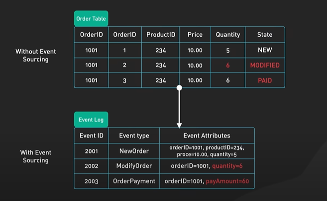
This approach provides a complete history of the system and enables better auditing and debugging.
Git version control is a great example of Event Sourcing, where each commit represents a change.
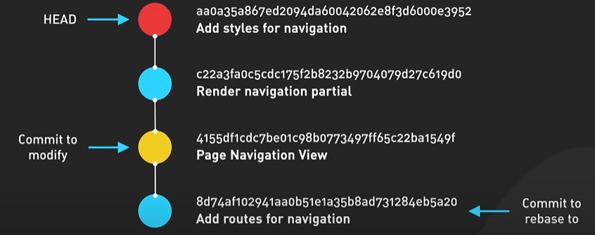
Event Sourcing, we can also implement advanced features like time-travel debugging or replaying events for analytics purposes.
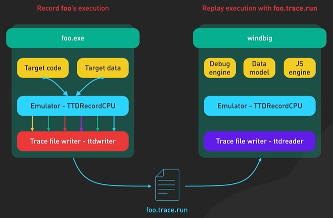
Leader Election - Imagine a classroom of students electing a class representative. In a distributed system, the Leader Election pattern ensures only one node is responsible for a specific task or resource. When a leader node fails, the remaining nodes elect a new leader.
ZooKeeper and etcd use this pattern to manage distributed configurations. By having a designated leader, we can avoid conflicts and ensure consistent decision-making across the distributed system.
PubSub - The Publisher/Subscriber pattern is like a newspaper delivery service.
Publishers emit events without knowing who’ll receive them, and subscribers listen for events they’re interested in. This pattern allows for better scalability and modularity.
For example, Google Cloud Pub/Sub enables asynchronous messaging between services, making it easier to maintain and scale complex applications.
Pub/Sub systems are well-suited for scenarios where we need to propagate changes or updates across multiple components, for example, updating a user’s profile across various services.
Sharding - Sharding is like dividing a large pizza into smaller slices, making it easier to handle. It’s a technique for distributing data across multiple nodes in a system. It improves performance and scalability. Each shard contains a subset of the data, reducing the load on any single node.
Databases like MongoDB and Cassandra use sharding to handle large amounts of data efficiently.
Sharding can also help us achieve better data locality, reducing network latency and speeding up query execution.
A bonus pattern - the Strangler Fig pattern.
This pattern is inspired by the strangler fig tree, which grows around other trees and eventually replaces them.
In software, the Strangler Fig pattern is a method for gradually replacing legacy systems with new implementations.
Instead of performing a risky “big bang” migration, we can incrementally replace parts of the old system with new components. This approach can help us manage the risks and complexities associated with system migrations.
Optimize SQL queries.
Query to find top 10 customer with the least of 1000 spend on order since Jan 2023 by joining the customer and order table and grouping by customer id. Display total order and amount spend sorted by desc order of total spend.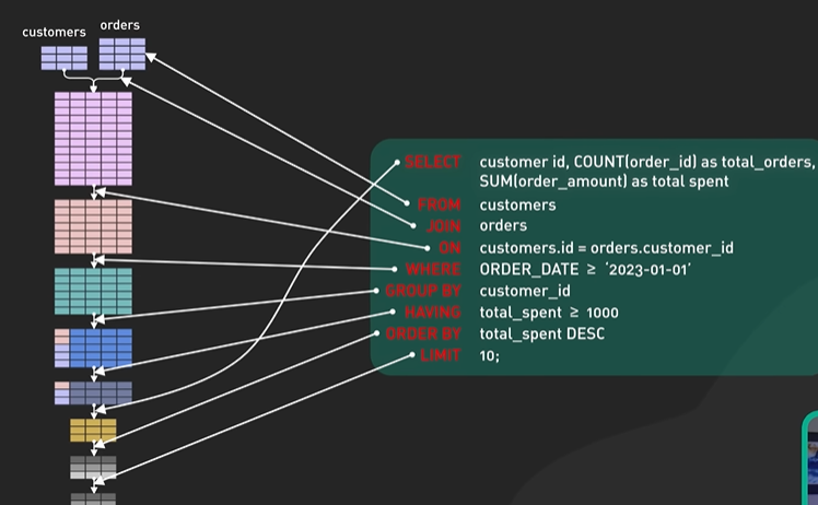
Database system creates those plans to optimize queries and minimize resource usage.
FROM and JOIN clauses - This is where we choose the table we will work with and specify how to join them.
Using index in join increase speed. Good index is the key. Index type like BitMap and B-Tree indexing can impact performance based on data distribution and query type.
WHERE - Conditions. Make the SARGABLE (Search Argument Able) query it indicate the faster execution.
When the query is SARGABLE then the query can be used to increase the speed of the index.
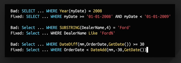
Sargable Query - WHERE order_date >= '2023-01-01'
Non-Sargable Query - WHERE YEAR(order_date) >= 2023
In Sargable query we directly compare order dtae column to a specific date. It allows db engine to use the index on the order_date column.
In Non query uses the YEAR function on the ORDER_DATE column and it prevent to use index in order date as teh function must be applied to every row in the table.
To write sargable queries -
Avoid using functions or calculations on indexed columns in the WHERE clause.
Use direct comparisons when possible instead of wrapping the column in a function.
If we need to use a function on a column, consider cresting a computed column or a function-based index, if the database system supports it.
GROUPBY and HAVING clauses.
To optimize SELECT clause consider using the index like SELECT, WHERE, JOIN. It enables teh db to retrieve data from the index.
ORDER_BY and LIMIT - To optimize use filtering and pagination. In large data set avoid sorting to large dataset as it reduce the response time.
The order is - FROM, JOIN, WHERE, GROUPBY, HAVING, SELECT, ORDER_BY, LIMIT.
Popular API Architecture Styles.
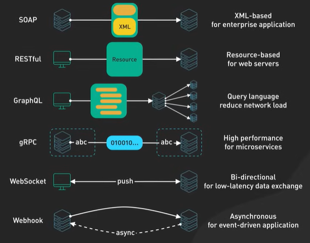
SOAP is used in financial services and payment gateway where the security and reliability are key.
REST is not suitable for real time data or operate with a highly connected data model.
GraphQL is not an architectural style and it is also a query language allows client to ask for a specific data. It means no over fetching or under fetching of data.
gRPC is modern, high performance and uses protocol buffers. It is used in microservice and Netflix uses gRPC to handle their immense inter-service communication. In browser client gRPC pose a issue due to limited browser support.
WebSocket is all about real time bidirectional and persistent connections.
Webhook is all about event driven, HTTP callbacks and asynchronous operation. Github uses webhooks to notify other systems whenever a new commit is pushed.
Most used Deployment Strategies.
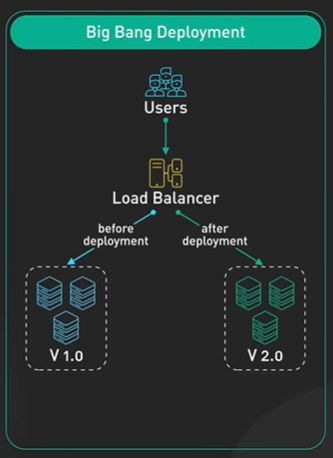
One of the earliest way to deploy into the production.
Push all the changes at once and it causes a bit of down time as we have to shut down the old system to switch to the new system.
It is sometimes the only choice in case of a database upgrade
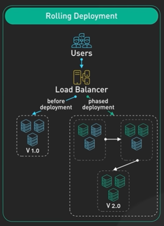
Rolling diplomat is more like a marathon than a sprint and this let us incrementally update different parts of the system over time.
Imagine there are 10 servers rolling deployment will take down the first server deploy the new version and continue with the rest of it 1 by 1. It prevents the downtown when one is updating and the other one is still working.
Maintaining two identical production environment like the blue and the green. At a given time one side is active and visible to the user and the other is idle.
The active one is serving the user and the ideal one is where we are doing the updates.
Canary deployment it is named after the ancient use of canaries in the coalmines. Update some of the server on particular location basis to see if that is working fine and monitor the performance of the new version.
Feature toggle is an option where you are making the user choose to update to the new feature or the previous one. Feature deployment can be used with any of the other deployment strategy.
How discord stores trillions of messages.
https://youtu.be/O3PwuzCvAjI?si=lOXYOAjxEg_jmNJ4
In this video, we’re going to discuss not just a database migration but a colossal task Discord engineers embarked on - moving trillions of messages from one database to another. If you’ve ever wondered what it takes to migrate data of such unimaginable scale, you’re gonna love this. Let’s dive right in. I’ve been eager to talk about this topic ever since I joined Discord. The engineering culture here is dynamic and innovative, and this story is a perfect illustration of that. Though this is all from public information, the insights and takeaways are my own. Discord recently peeled back the curtain on how they migrated trillions of messages from Cassandra - the database that houses your chats and conversations, to ScyllaDB - a faster and more reliable alternative. The process was first shared at ScyllaDB Summit 2023 by Bo Ingram, followed by a detailed blog post. A big shout-out to Bo for presenting this complex process so clearly. So, what did Bo share? I’ll summarize and share my own takeaways. You can watch his video and read his blog post if you want to learn more about it. Let’s rewind back a few years. Discord found themselves in a bit of a pickle with their database choice. They were using Cassandra, but as the platform continued to grow, they faced serious performance issues. It took a lot of effort to maintain the main Cassandra cluster that held messages. The latency was unpredictable, and the frequent on-call incidents put huge strain on the team. By 2022, the Cassandra cluster held trillions of messages across 177 nodes. They knew they needed something different, but this message cluster was critical to Discord. If the message cluster is slow, Discord is going to be slow. If the message cluster is down, Discord is going to be down. Their solution? ScyllaDB, a Cassandra-compatible database, but with a more powerful C++ based engine under the hood. Instead of jumping in headfirst to solve the riskiest and biggest problem, they started the migration with smaller databases. And this is my first takeaway. At Discord, the engineers move fast when mistakes are reversible, but if the solution is a one-way door, they spend a lot more time and care to get it right. They used these small migrations as an opportunity to test the waters and iron out as many issues as possible before tackling the big beast that held trillions of messages. Let’s talk a bit about ScyllaDB. It was written in C++ and promised better performance, faster repairs, and most importantly, it was garbage collection-free. For a team that had so many issues with Cassandra’s garbage collector, this was a breath of fresh air. The next key step was to create an intermediate layer between the API monolith and the database clusters called data services. The layer was written in Rust, which is a safe and highly performant language. And it’s a joy to write in Rust. The really cool idea about this layer is something called request coalescing. If multiple users request the same data, the database only needs to be queried once. This drastically reduced the potential for hot partitions. Imagine all those unintended @everyone messages in hugely popular discord servers. With this layer in between, it is no problem for the database at all. Then, they came up with the concept of a Super-Disk. The database clusters run on Google Cloud. When faced with the challenges of disk latency, they couldn’t rely on the local NVMe SSDs on the virtual machines for their critical data storage due to reliability and durability issues. The alternative was Google Cloud’s Persistent Disks. While it was reliable and flexible, it had the disadvantage of higher latency since they were network-attached rather than directly attached. So, what did Discord do? They went back to the drawing board and focused on creating a solution tailored to their specific needs. They chose to prioritize low-latency disk reads over all other disk metrics while maintaining the existing database uptime guarantee. What they came up with was a super-disk combining the best of local SSDs and Persistent Disks at the software level. Their super-disk was a two-layered RAID solution. They used RAID0 to combine multiple Local SSDs into one low-latency virtual disk, and then RAID1 to mirror this RAID0 array with a Persistent Disk. They then configured the linux kernel to direct the write to the persistent disk, which had strong durability guarantee, and the read to the local SSDs, which offered low latency. This setup ensured low-latency reads from the Local SSDs and write durability from the Persistent Disks. What’s so great about this? It’s an excellent example of problem-solving from first principles. Discord was dealing with a problem that had no ready-made solution. Instead of trying to make do with what was available, they redefined the problem based on their specific needs and then built a solution to match. The super-disk worked. At peak load, the databases no longer started queueing up disk operations, and they saw no change in query latency. Finally, with all this prep work done, it was time to migrate their largest database - the ‘cassandra-messages’ cluster. With trillions of messages and nearly 200 nodes, it was a daunting task. But with a newly written data migrator in Rust and some clever strategies, they managed to do it in just nine days! Yes, you heard that right - they migrated trillions of messages with NO downtime in less than two weeks! And the payoff? A significantly quieter, more efficient system. They went from running 177 Cassandra nodes to just 72 ScyllaDB nodes. It drastically improved latencies and the quality of life for the on-call staff. It was no ordinary task, but with clever risk mitigation and innovative solutions, they pulled it off. So there you have it. I’m incredibly proud of what the team was able to pull off. Migrating a production database is no joke, and doing it at this scale… well, it is hard. If you like our videos, you may like our system design newsletter as well.
Stack overflow Architecture.
https://youtu.be/fKc050dvNIE?si=JhzCzmkAsuOiA2ns
You might think you’ve cracked the code to designing a platform that serves 2 billion page views a month, but what Stack Overflow does in reality might surprise you. Imagine being tasked with designing the Stack Overflow website. You suggest on-premise servers and a monolithic application, only to get raised eyebrows from your fellow engineers. Yet, this is precisely how Stack Overflow functions. You’d expect a platform like Stack Overflow to mimic prevailing trends. A typical big-tech software engineer might sketch a system with microservices, breaking the system into manageable chunks, each with its own database. They’d show extensive use of caching, sharded services, and asynchronous communication through message queues. Some might even show off a bit with Event Sourcing paired with CQRS. And who wouldn’t seize the chance to sprinkle in some distributed system concepts like eventual consistency and the CAP theorem? Impressive, right? But here’s the twist. None of these elements feature in Stack Overflow’s design. In a tech world saturated with microservices, Kubernetes, and cloud-based solutions, Stack Overflow stands as an anomaly. Instead of following trends, they’ve stuck to an architecture that best fits their unique circumstances. With a single monolithic application handling the main Q&A sites, they challenge our preconceptions about designing large-scale systems. Against popular belief, Stack Overflow operates with a monolithic application running on just nine on-premise web servers. They don’t rely on the cloud or break their application into microservices, yet they efficiently handle tremendous traffic with their unconventional approach. Instead of planning for relentless change, they’ve designed a system optimized for low latency and memory allocation. These servers run at a comfortable 5 to 10% capacity, leaving plenty of space for growth. Despite 80% of their traffic being anonymous - users who land, find their solution, and leave - they maintain an astonishing performance. Even their most-visited page, the question show page, is not cached, yet it renders in a swift 20 milliseconds. This exceptional performance is powered by a massive 1.5 terabytes of RAM on their SQL Server instances, enabling fast access to a third of their entire database in memory. Their success prompts us to question: What if the most hyped tech concepts aren’t always the best solution? What if the key to robust system design lies in a deeper understanding of specific challenges, rather than chasing the latest trends? Stack Overflow’s story is a striking case study that reminds us that technology isn’t a one-size-fits-all field. What works for one may not work for another, emphasizing the need to align system architecture with specific business and technical needs rather than blindly following industry trends. Stack Overflow’s tale is one of efficiency, practicality, and defying stereotypes - a true testament to the power of thinking outside the box.
OAuth 2.
https://youtu.be/ZV5yTm4pT8g?si=VBty5SJ9UgjeemVL
around o off2 but ended up lost in the sea of jargons that’s why we’re here today we’re breaking down these complex Concepts into digestible explanations let’s Dive Right In imagine the early days of the internet sharing info was straightforward just hand over your username and password to another service and they could access anything they wanted this practice is fry upon these days but we might still encounter this practice in certain personal finance software to scrape information from crusto Banks luckily we have something much better these days enter OA 2 OA 2 is like giving someone a special key this key allows them to access specific information in another application we control who gets access to our data without having to share a password and yes we can revoke that key at any time now let’s play this out with an example consider a photo storage application Snap Store we’ve been using it to store our photos and now we want to print some of them using a thirdparty printing service PR magic instead of manually uploading each photo to PR magic we ask PR magic to do the job with a simple click we Grant PR magic permission to access our photos on Snap Store using o Off 2 preager can then access our Snap Store photos on our behalf without ever knowing our Snap Store login credentials this is an example of the O off flow is an elegant stance between us Prem magic and snap store all orchestrated by o of2 now let’s unpack this further in this context we are the resource owner because we own our photos on Snap Store Snap Store is the resource server that stores our photos pre magic is the client that wants to access the photos the authorization server could be a part of snap store or an external identity provider and is responsible for handling the O off2 process let’s follow the oof2 flow in this scenario it begins when we instruct pre magic to fetch photos from Snap Store pre magic sends a client ID and scope which represent the access level requested to snap store’s authorization server as a resource owner we authenticate directly with SNAP store and Grant Prem magic the consent to access our photos once consent is granted the authorization server sends an authorization code back to PR magic Prim magic then presents this authorization code is client ID and client secret to the authorization server now the client secret is a private key shared only between PR magic and the authorization server if the authorization server verifies the authorization code client ID and client secret IT issues an access token to PR magic finally Prim magic uses this access token to request our photos from snap store’s resource server this all off to process ensures that our Snap Store login credentials are never exposed to pre magic while allowing pre magic to access only the photos we authorized it to see it’s also important to note that the access token can be set to expire after a certain time or can be revoked by us at any point providing an additional layer of security oa2 also support refresh tokens which can be used to obtain a new access token when the o one expires without requiring our in ition that’s o off to in a nutshell is an essential piece of the web security infrastructure and the backbone of many secure Seamless app interactions we use daily if you like our videos you may
Netflix API Architecture.
https://youtu.be/Uu32ggF-DWg?si=FlEftahR9cwTElna
Have you ever wondered about the technology that underpins its operations to allow them to create this massive library? Today, we’re going to explore the remarkable journey of Netflix’s studio-facing API architecture. In the early days, Netflix employed a monolithic architecture. Just picture a massive, interconnected system where all components were part of one unified codebase. As Netflix grew and collaborated with more studios to create original content, this monolith started to become a roadblock rather than a solution. So, what’s the next move? Netflix engineers carved up the monolith into microservices. Netflix is known for having a massive number of these services. This shift led to increased efficiency and autonomy. It transformed their architecture into a web of services. But directly interfacing the applications that studios use with so many microservices was far from ideal. To overcome this challenge, they introduced a gateway aggregation layer. They essentially built an API Gateway to bind all the services together and presented a unified front to the clients. This setup worked great for use cases that span multiple services. Imagine the studio app needs 3 APIs, say movie, production, and talent, to render the frontend UI. The gateway aggregation layer makes this possible. The gateway aggregation layer was supposed to bring order, but instead it became the new monolith as the team grew and services multiplied. As the number of developers grew and domain complexity increased, developing the gateway aggregation layer became increasingly difficult. To resolve this, Netflix turned to GraphQL and introduced the Federated Gateway. This strategy allowed domain experts to manage their own part of the ‘graph’, while providing a unified, efficient access point for various studio applications. GraphQL is the heart of the Federated Gateway. This powerful query language enables the UI to fetch exactly what it needs in a single round trip, even when the user is far from the datacenter. Thanks to GraphQL and the Federated Gateway, Netflix was able to route complex business logic directly to the appropriate services. GraphQL federation allows Netflix to set up a single GraphQL gateway that fetches data from all the other APIs. This journey from monolith to federated gateway illustrates how system architecture needs to adapt to growing and dynamic business needs. It’s these behind-the-scenes adaptations that enable Netflix to create the content we all enjoy. But here’s the main takeaway. The evolution of architecture is key. It’s easy to look at giants like Google and Netflix and want to replicate their infrastructure, even when it’s not necessary. Over-optimizing for problems you don’t have, and might never have, is a common pitfall." Instead, we need to focus on our unique needs. We should decide where our business logic should reside, and identify where we’ll need to scale as our business grows. The architecture of our business should be tailored to its needs, not the other way around. The best architecture is the one that fits our business needs, not one that mimics the tech giants. If you like our videos, you may like our system design newsletter as well.
DevOps SRE Platform Engineering.
DevOps, coined by Patrick Debois and Andrew Shafer in 2009. DevOps is all about bridging the gap between two traditionally separate teams - Development and Operations.
A cloud engineer bootstrapping a virtual instance with Ansible and running Kubernetes on top might look like a DevOps specialist. Similarly, a sysadmin building tools and utilizing monitoring system could be considered an SRE.
Site Reliability Engineering. A brainchild of Google, SRE is about building resilience into large, complex systems. They developed practices and tools, like Borg cluster management system and Monarch monitoring system, to ensure that software can handle the stress of real-world demands.
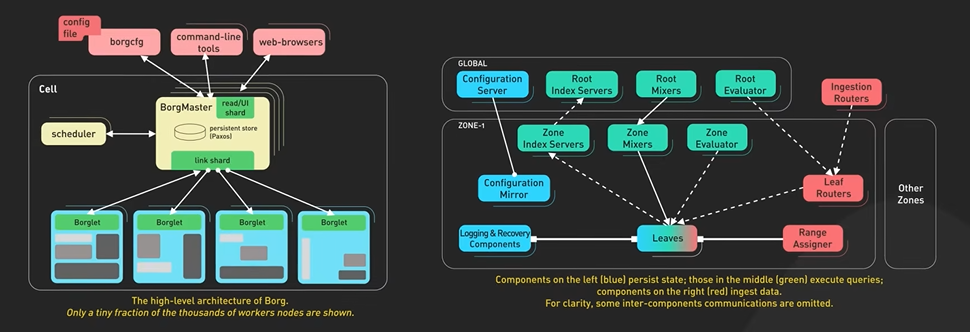
They sometimes build tools to simplify processes for developers, stepping into the territory of a Platform Engineer.
So, what exactly is Platform Engineering? What does it look like in action?
A great example is Netflix. Netflix is well known for its cutting edge infrastructure. A key player to this is its Platform Engineering team. They develop a solid, reliable platform that enables developers to produce high-quality software quickly. But it’s not just about the technology. It’s about aligning the entire lifecycle of product development with broader business objectives.
It serves as the connective tissue and binds the different components of software development and operations into a cohesive unit.
DevOps, SRE, and Platform Engineering share a common vision: to enhance collaboration, automation, and efficiency in software development and operations.
Improve API performance.
API first need to see the bottleneck by load testing and profiling request. Optimization should only be done when the API has some performance issue.
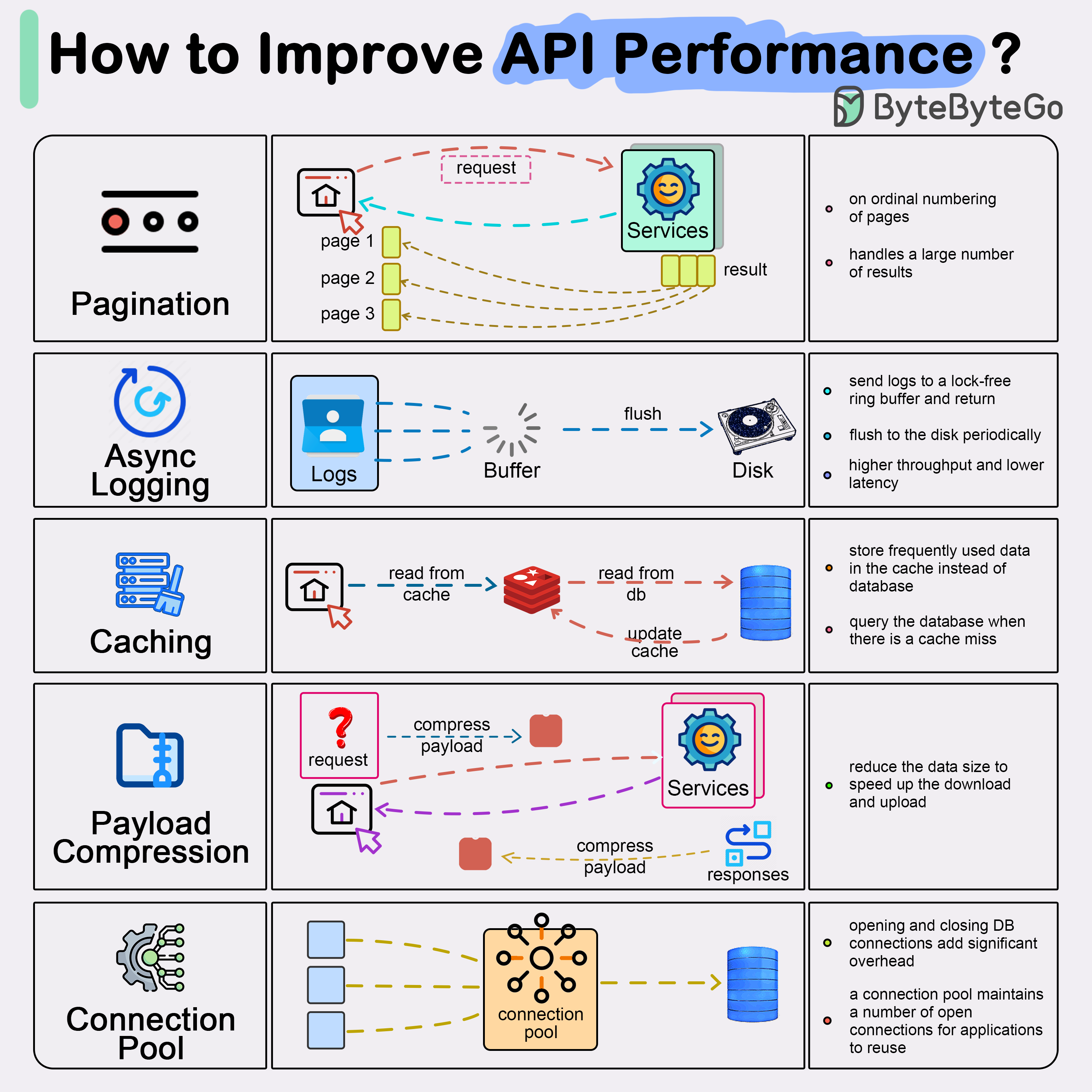
Connection Pooling - This technique involves using a pool of open connections to manage database interaction, which reduces the overhead associated with opening and closing connections each time data needs to be loaded. The pool manages the lifecycle of connections for efficient resource use. Creating a connection uses a handshake protocol and slow down the API. The reuse of connection can greatly improve throughput.
In serverless architecture the connection management is a bit more challenging. Each serverless function instance opens its own database connection. Serverless can scale rapidly and it can potentially lead to a large number of open connections and that can overwhelm the database.
AWS RDS proxy and Azure SQL database are designed to handle the situation and manage the connection pooling for you.
Avoid N+1 query problem.
It optimizes the db performance.
Example building an API endpoint to fetch a blog post their comments. The N+1 problem will occur when we first make a query to fetch the post and for each post another query to fetch the comments.
SELECT id, title FROM posts;

SELECT id, content FROM comments WHERE id=1;
SELECT id, content FROM comments WHERE id=2;
SELECT id, content FROM comments WHERE id=3;
There are N post and then there will be 1 query for the post and N queries for the comments - N+1 problem.
To avoid this fetch the data in a single queries or two queries . One to fetch the post and one to fetch all the comments for those posts.
SELECT posts.id AS post_id, posts_title, comments.id AS comment_id, comments.conten AS comment_content FROM posts LEFT JOIN comments ON comments.post_id = posts.id;
Use pagination.
Using lightweight JSON serializer.
When returning JSON responses the speed of the serializer can make impact in response time.
Compression.
Enabling compression on large API response payload can reduce the amount of data transfer over the network.
Why Google Mono repo.
https://youtu.be/x3cANGNPyx0?si=9PNb6l6O4P1Pro_i
manage to keep their mountains of code in check? Or perhaps we’re deciding how best to structure our own project’s code? The way we manage our code can make or break the team’s productivity and the product’s stability. That’s why today, we’re diving into the great repository debate: monorepos versus microrepos. Before we dive in, did you know that the monorepo concept isn’t new? Both Linux and Windows were created using a monorepo approach. Monorepo Overview Let’s start with monorepos. Think of it as one central hub where all our code lives. Companies like Google, Facebook, and Uber - they’ve chosen the monorepo path. It’s like a giant library - perhaps a bit daunting to navigate, but everything’s under one roof. Let’s kick things off with monorepos. Picture it like a vast library where every single line of code we’ve ever written lives. Companies like Google, Facebook, and Uber - they’ve gone down the monorepo route. Just imagine - in Google’s monorepo, there are billions of lines of code, all under one roof! Sounds pretty intense, right? Let’s go through the pros and cons of monorepos. Pros: Here’s one clear benefit of a monorepo: making cross-project changes becomes a breeze. Let’s say we have a utility function that’s used in 10 different services, and we need to make a change. In a monorepo, we can do this in one commit, in one place. Then there’s dependency management. Instead of wrestling with multiple versions of a package across different repositories, we’ve got a single, consolidated view of our dependencies. Consistency is another big win for monorepos. You know how code reviews sometimes feel like the Wild West, with different rules and standards across teams? Well, with a monorepo, everyone’s playing by the same rules. And don’t forget code reuse. Need a functionality that’s already been developed for another service? No need to recreate the wheel. We can see everything in the monorepo, making it straightforward to repurpose code. Cons: However, it’s not without challenges. Monorepos require careful planning and the right tools. Google even had to build a dedicated tool called Blaze and staff a large team to support their massive codebase. Facebook uses Buck for similar reasons. And as the repository grows, without careful management, the CI/CD pipelines might start moving at a snail’s pace. This is another area that requires a heavy level of staffing. And for the new developers, a large repository can be overwhelming. But with a well-documented codebase and structured onboarding process, even the largest monorepo can become manageable. Lastly, although each team ‘owns’ a section of the monorepo, customization can be tricky. Teams can’t always independently use different tools or libraries due to possible conflicts, and major changes need to consider the entire codebase. That said, using tools like Google’s Bazel and maintaining good communication can help balance this trade-off, allowing teams to flexibly evolve within shared guidelines. Microrepo Overview: Now, let’s switch gears to microrepos. This approach treats each component or service as an independent entity, with its own separate repository. Organizations such as Amazon and Netflix have embraced this decentralized method. Let’s walk through the pros and cons. Pros: Microrepos offer independence. Each team can manage and scale their repos as needed. Another advantage is risk isolation. If something goes wrong in one repo, it doesn’t affect the others, reducing the blast radius. This approach also provides flexibility. Each team can select the best tools for their repo and tailor their environment to their exact needs. And there’s a clear sense of ownership - each team manages their own repository." Cons: However, there are downsides. Coordinating changes across multiple repos can be challenging. It requires solid collaboration and possibly specialized tooling Managing dependencies across many repos can be challenging. But tools like Nexus or Artifactory can help. Without a unified standard, code standards can vary widely. This can lead to poor code quality or inconsistent patterns. To prevent this, it’s important to establish organization-wide coding guidelines. And one more thing - code duplication. Copying the same code across repos bloats the codebase and can lead to bugs. To avoid this, creating shared libraries for common code can be useful. Which is Better? So, the big question: monorepo or microrepos? Well, as with many things in tech, it’s not black and white. The best approach depends on factors like the team’s needs, the size of the organization, the nature of the projects, and the company’s culture. Monorepos bring consistency, make cross-project changes smoother, and promote code reuse. They’re a great fit if we have large teams working on interconnected projects where collaboration and consistency are key. But remember, they require careful upfront planning and tooling. Unmanaged, they can affect the performance of the CI/CD pipelines and offer less flexibility to individual teams. On the flip side, microrepos offer flexibility, risk isolation, and clear ownership. They can be a good choice for organizations that prioritize team autonomy, especially if teams are working on distinct projects. But, they come with their own challenges. They can be more complex to manage, especially when making cross-repo changes, and may lead to code duplication if not managed well. So, what works best for you? Share your chosen strategy in the comments, and let us know why you opted for it. Looking forward to hearing your experiences with monorepos and microrepos. If you like our videos, you may like our system design newsletter as well. It covers topics and trends in large-scale system design. Trusted by 450,000 readers. Subscribe at blog.bytebytego.com
Git Merge VS Rebase.
https://youtu.be/0chZFIZLR_0?si=vdKjmcm6JDOYo14B
Hey there! Have you ever been stuck, not sure whether to use git merge, git rebase, or squash your commits? Trust me, you’re not the only one! Today, we’re going to tackle these sometimes puzzling Git topics. We’ll break down the key differences between these Git commands and when to use each for our workflow. If you’ve ever worked on a Git project with a bunch of branches, you’ve probably had to figure out how to get changes from a feature branch back into the main branch, or keep your feature branch up to date with the main branch. The big question is, should we use git merge, git rebase, or squash our commits? Let’s pull back the curtain and see what’s really going on with each one. Main content So, let’s say we’ve created a new feature branch from main. We’ve added commits A, B, and C on the feature branch. At the same time, the main branch has added commits D and E. Picture it like two branches of a tree, growing in different directions. Keeping our feature branch up to date with main is a crucial part of the Git workflow. We can do this with either git merge or git rebase. Here’s what that means: “git merge” pulls in the latest changes from main into the feature branch, creating a new “merge commit” in the process. It’s like tying the two branches together with a knot. “git rebase” changes the base of our feature branch to the latest commit on main and then replays our changes from there. It gives us a clean, straightforward commit history, which many people prefer. Now, once we’ve finished developing the feature, we’ll want to get the feature branch back into the main branch. We have a few options for this: First is Git Merge. Git will create a new “merge commit” that ties together the histories of both branches. It’s like creating a knot in the rope that shows where the branches joined. But if we do this a lot, we end up with lots of knots, which can make the history a bit messy. Another option is “Git Rebase and Fast-Forward Merge”. We can use git rebase to move our feature branch’s changes onto the tip of main, and then perform a fast-forward merge. This is like straightening out the rope so it’s all in one line. Squash Commits: With squashing, all the feature branch commits are squeezed into a single commit when merged into main. This keeps main’s history linear like rebasing, while still creating a single merge commit. But remember, we lose the fine details of individual feature commits in the main branch’s commit history. That said, squashing commits is a popular strategy on platforms like GitHub because it allows us to tidy up history in the main branch while still preserving the detailed commit history in the feature branch. It’s a kind of a hybrid approach! To sum it up, “git merge” gives us a complete picture of the commit history and branch evolution. “Git rebase” tidies up history by moving commits to the main branch tip. Squashing commits consolidates commits into one, providing a clean, linear history in the main branch but at the cost of detailed commit history. Now, imagine a scenario where the team values a clean, straightforward history but doesn’t mind losing the detailed history of individual commits within the main branch. In this case, squashing commits might be the way to go. But remember, it’s all about assessing the pros and cons and deciding which workflow makes the most sense for the team. There’s no one-size-fits-all approach - it all comes down to what you value most. If you like our videos, you may like our system design newsletter as well. It covers topics and
Top 6 load balancing algorithms.
https://youtu.be/dBmxNsS3BGE?si=xi8-0pownu9m7wH8
handle millions of requests without breaking a sweat? Load balancing is an absolutely critical component of any large-scale web application. By distributing workload across multiple servers, load balancing helps ensure high availability, responsiveness, and scalability. Understanding the core load balancing algorithms will allow us to better architect, troubleshoot, and optimize our applications. There are two main categories of algorithms: static and dynamic. We’ll provide an overview of each category and dive deeper into the major specific algorithms, including how they work and their pros and cons. Stick around to the end because we’ll also summarize key criteria to help you select the right algorithm. Let’s get started! Static load balancing algorithms distribute requests to servers without taking into account the servers’ real-time conditions and performance metrics. The main advantage is simplicity, but the downside is less adaptability and precision. Round robin is conceptually the simplest approach. It rotates requests evenly among the servers, sending request 1 to server A, request 2 to server B, and so on in sequence. This algorithm is easy to implement and understand. However, it can potentially overload servers if they are not properly monitored. Sticky round robin is an extension of round robin that tries to send subsequent requests from the same user to the same server. The goal here is to improve performance by having related data on the same server. But uneven loads can easily occur since newly arriving users are assigned randomly. Weighted round robin allows admins to assign different weights or priorities to different servers. Servers with higher weights will receive a proportionally higher number of requests. This allows us to account for heterogeneous server capabilities. The downside is that the weights must be manually configured, which is less adaptive to real-time changes. Hash-based algorithms use a hash function to map incoming requests to the backend servers. The hash function often uses the client’s IP address or the requested URL as input for determining where to route each request. It can evenly distribute requests if the function is chosen wisely. However, selecting an optimal hash function could be challenging. Now let’s switch gears to dynamic load balancing algorithms. These adapt in real-time by taking active performance metrics and server conditions into account when distributing requests. Least connections algorithms send each new request to the server currently with the least number of active connections or open requests. This requires actively tracking the number of ongoing connections on each backend server. The advantage is new requests are adaptively routed to where there is most remaining capacity. However, it’s possible for load to unintentionally concentrate on certain servers if connections pile up unevenly. Least response time algorithms send incoming requests to the server with the lowest current latency or fastest response time. Latency for each server is continuously measured and factored in. This approach is highly adaptive and reactive. However, it requires constant monitoring which incurs significant overhead and introduces complexity. It also doesn’t consider how many existing requests each server already has. So in summary, there are clear tradeoffs between simpler static algorithms and more adaptive dynamic ones. Think about our specific performance goals, capabilities, and constraints when selecting a load balancing strategy. Static algorithms like round robin work well for stateless applications. Dynamic algorithms help optimize response times and availability for large, complex applications. Also, the differentiation between “static” and “dynamic” is somewhat simplified. Which algorithms do you think suits your needs best? Have you faced any challenges with load balancing in the past? Share your experiences and insights in the comments below. We’d love to learn from you, and we’ll see you in our next video. If you like our videos, you may like our system design newsletter as well. It covers topics and trends in large-scale system design. Trusted by 500,000 readers. Subscribe at blog.bytebytego.com
Algorithm in System Design.
https://youtu.be/xbgzl2maQUU?si=jqLwqXhKUI8Tp-re
Hey there! In today’s video, we’ll dive into some key algorithms that you should know as a software engineer. These algorithms aren’t just useful for acing system design interviews - they’re also great tools for building real-world systems. We won’t be digging into implementation details here. Instead, we’ll focus on why these algorithms matter and where we might use them. Understanding the high-level concepts is more important than memorizing code for interviews. Let’s see how many of these you already know! First up, consistent hashing. Ever wondered how systems like Cassandra distribute data across multiple servers? They use this algorithm. Picture a ring where each key, after hashing, maps to a point on it. Servers are assigned ranges on this ring. This means that when adding or removing servers, only keys in the affected ranges need remapping. This is way better than naive hash mappings that would require remapping all keys when servers change. One cool idea here is the use of virtual nodes. It helps to tackle non-uniform data distribution. Check out variants like rendezvous hashing or jump consistent hashing if you want to dig deeper. If you’re into distributed caching or databases, consistent hashing is great to know. In the era of big data, ensuring efficient data distribution is crucial. Consistent hashing minimizes disruptions as servers come and go. Next let’s talk about quadtrees for spatial indexing. Quadtrees work by recursively subdividing 2D space into 4 quadrants. Each node represents a region, and has 0 to 4 child nodes. Why quadtrees? They enable fast location-based insertion and searches. We can quickly find points in a radius by traversing the tree and pruning branches outside the range. This makes quadtrees ideal for indexing spatial data used in mapping apps. Quadtrees are flexible and effective for 2D spatial indexing. Check out other spatial indexing trees like R-trees and KD-trees if you want to learn more. Now let’s look at the leaky bucket algorithm for rate limiting. Imagine a bucket with a tiny hole at the bottom - that’s our leaky bucket. Requests pour in like water, but if the bucket’s full, they’re turned away until there’s room again. Setting it up is simple. The bucket size controls burst capacity. It leaks at whatever rate we set. Each request is like adding a drop of water. If it’s overflowing, requests have to wait. There’s other rate limiting algorithms - like token bucket and sliding window counter. They are simple and effective algorithms, with each making tradeoffs between accuracy and performance. Next up - tries, a tree structure optimized for storing strings and prefixes. Each node represents a common prefix, with nodes sharing prefixes using the same subtree. The real power of tries lies in fast lookup speed. Searches are super efficient. Imagine searching for a word or a prefix in a large dataset. With tries, we don’t need to sift through every entry. Instead, the search elegantly progresses through the tree, moving character by character, following branches that match the search term. This makes operations like autocomplete in search engines or text editors lightning fast, way faster than with structures like hash tables or arrays. One catch - they can be a bit greedy with memory. This is because each node often maintains multiple child pointers. There are variants like radix tries or suffix tries that optimize memory usage. Tries are a powerful foundation for scalable string-based searches. Next, we have Bloom filters. These are a probabilistic data structure for set membership checks. Picture a bit array combined with some hash functions. Items get hashed and their corresponding bits set. To check membership, we see if all the bits are set. If not all set? Definitely not in the set. All set? Maybe in the set, but watch out for false positives. We can’t remove elements once added. And what about those false positives? We can tweak things like size or hash functions to balance space and accuracy. Bloom filters shine in caching, deduplication, and analytics by quickly filtering out noise. Last but not least, let’s talk about consensus algorithms. In distributed systems, reaching consensus, that is, ensuring all nodes consistently agree on a shared state, is tricky, especially with network issues and failures. Algorithms like Paxos and Raft are designed to address this challenge. Let’s focus on Raft since it shines through its simplicity and efficiency. Raft elects a leader to manage state replication across the cluster. If nodes fail, Raft ensures the system stays operational to prevent inconsistent data and downtime. A major plus is that it’s easy to understand and implement. Many distributed systems like Kafka and etcd have adopted Raft for replication, failover, and leader election. Paxos predates Raft and is historically significant but more complex. And there you have it! A quick tour of the WHYs behind some essential algorithms. What other real-world applications have you seen or used these algorithms in? Drop a comment below. Let us know if you have any other algorithms you find useful as an engineer.
Most used Architecture Patterns.
https://youtu.be/f6zXyq4VPP8?si=CVJ3E2mx-eLjaMFz
Software architecture is to applications what foundations are to buildings. Build it wrong, and no matter how beautiful it looks, it’ll crumble. In today’s discussion, we’ll unpack some prevalent software architecture patterns that form the backbone of countless applications and platforms we interact with daily. Over the next few minutes, we’ll explore five key patterns that have shaped the industry. Let’s start with layered architecture. This pattern separates the components of a system into distinct layers, typically the presentation layer, business logic layer, and data access layer. For instance, in user interface design, we often see the Model-View-Presenter (MVP) pattern. It is a specialized form of layered architecture. Here, the Model represents data and business logic, the View displays this data, and the Presenter serves as a bridge to ensure a clean separation of concerns. The primary goal of layered architectures is to promote separation so changes in one layer don’t negatively impact others. This structure provides abstraction and encapsulation, with each layer having a distinct responsibility. Next is event-driven architecture. This pattern promotes the production and consumption of events between loosely coupled software components and services. Components broadcast events when something notable happens, and other components subscribe to specific events they are interested in. This allows for highly decoupled architectures. One prominent example in this domain is Command Query Responsibility Segregation (CQRS). With CQRS, the data write operations (commands) are separated from read operations (queries), and changes are often communicated through events. This makes the system inherently event-driven. The pub/sub model, where components publish and subscribe to events, is commonly used in such architectures. Here, components don’t call each other directly; they merely react to published events. Moving on to microkernel architecture. This pattern emphasizes separating core system functionality into a small microkernel and extended functionality into add-ons or plugins. In operating systems, for example, a microkernel might oversee vital tasks like inter-process communication while offloading other system functions to external components. An application example is the Eclipse IDE: its core runtime handles the plugin architecture, and features from Java tools to Git integration are delivered as plugins. This design prioritizes extensibility, ease of maintenance, and fault isolation. Whether it’s an OS component or an Eclipse plugin that encounters an issue, the core system remains stable and unaffected. Then we have microservices architecture. This decomposes an application into a collection of small, loosely coupled services. Each service implements specific business capabilities, contains its own data model, and communicates via APIs. Netflix, for instance, uses microservices to handle everything from movie recommendations to billing. This architecture promotes modularization of functionality so services can be developed, deployed, and scaled independently. It increases agility, and allows companies like Netflix to rapidly innovate. The trade-off, however, is the added complexity in managing inter-service communication and maintaining data consistency. Last but certainly not least, we have monolithic architecture. At its core, a monolithic design sees all components of the application — from data access and business logic to the user interface — bundled together into a single codebase and run as a single unit. This approach simplifies development and deployment, making it a go-to for many startups and smaller applications. However, it’s worth noting the rise of the ‘modular monolith’. This approach retains the benefits of a single deployable unit but emphasizes clear modular boundaries within the codebase. This allows for easier maintenance and scalability. It’s a middle ground which offers the simplicity of a monolith while paving the way for potential future transitions to architectures like microservices. Regardless of the approach, many successful platforms start with a monolithic or modular monolithic structure before considering more distributed architectures. And there you have it, a quick tour of five foundational software architecture patterns. The right choice always depends on our specific challenges, requirements, and contexts. So, which pattern resonates with you? Drop a comment below and let us know which architecture pattern intrigues you the most. If you like our videos, you may like our system design newsletter as well. It covers topics and trends in large-scale system design. Trusted by 500,000 readers. Subscribe at blog.bytebytego.com
Apache Kafka.
Originally developed at LinkedIn, Kafka was created to solve the problem of ingesting high volumes of event data with low latency. It was open-sourced in 2011 through the Apache Software Foundation and has since become one of the most popular event streaming platforms.
Event streams are organized into topics that are distributed across multiple servers called brokers. This ensures data is easily accessible and resilient to system crashes.
Kafka Use Cases.
First, Kafka serves as a highly reliable, scalable message queue. It decouples data producers from data consumers, which allows them to operate independently and efficiently at scale.
A major use case is activity tracking. Kafka is ideal for ingesting and storing real-time events like clicks, views and purchases from high traffic websites and applications.
In microservices architecture, Kafka serves as the real-time data bus that allows different services to talk to each other.
Kafka is also great for monitoring and observability when integrated with the ELK stack. It collects metrics, application logs and network data in real-time, which can then be aggregated and analyzed to monitor overall system health and performance.
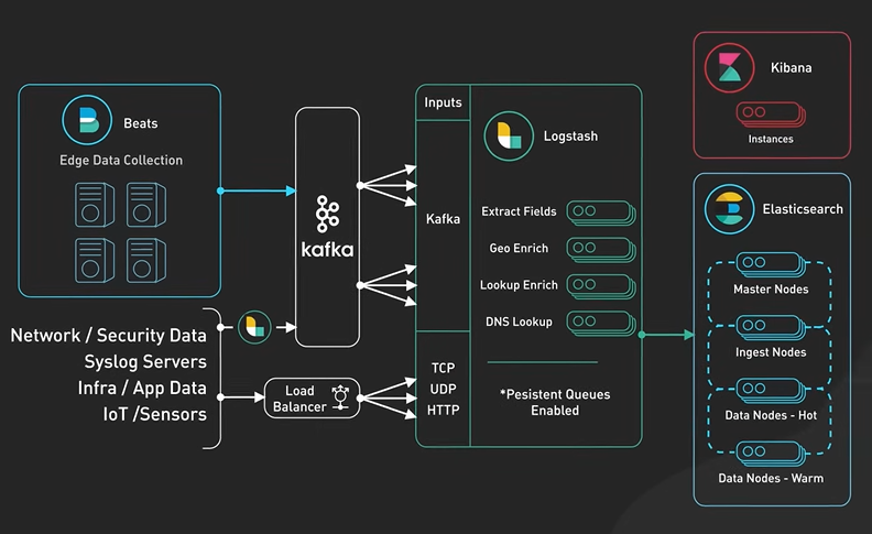
Kafka enables scalable stream processing of big data through its distributed architecture. It can handle massive volume of real-time data streams.
Kafka has some limitations though. It is quite complicated. It has a steep learning curve. It requires some expertise for setup, scaling, and maintenance. It can be quite resource-intensive, requiring substantial hardware and operational investment. It is also not suitable for ultra-low-latency applications like high frequency trading, where microseconds matter.
System Design Interview.
https://youtu.be/o-k7h2G3Gco?si=uCjlGt60rKfwMnbb
Hey there! This is Sahn. In today’s video, I’m going to share with you our proven strategies for crushing your system design interviews. Having interviewed countless candidates, I’ve seen up close what works and what falls short when it comes to preparing for these tough interviews. Stick with me for the next few minutes, and I’ll guide you through a preparation approach that’ll have you tackling any system design question with confidence. Let’s dive right in! First off, you might be wondering: what is a system design interview? At a high level, its purpose is to assess your ability to: One, translate an ambiguous problem statement into concrete technical requirements. Two, craft an architecture and design that satisfies those requirements. Three, articulate and defend your design decisions throughout the discussion. You’ll be asked to design large scale systems like an Instagram feed, Uber ride sharing, Twitter timelines, or even the infrastructure behind Google Search. Remember, there’s no such thing as the “right” or “perfect” solution. The goal is to demonstrate your technical expertise, your approach to problem solving, and your skills to communicate effectively. Now, you may be wondering - why should we care about preparing for system design questions? What’s the big deal? Well, here’s the main reason: Your performance in a system design interview can often determine whether you land a senior engineer position, or if you’re considered for a more junior role. Once you’ve clocked in a few years in the industry, system design is how companies gauge your ability to build complex systems at scale. Essentially, shine bright in the system design interview, and you’re on track for those senior titles. But if you hit bumps along the way, you could be looking at offers for more junior positions. So it pays to put in the work and take these interviews seriously. You might be thinking: How on earth can these companies assess our abilities in such a short period of time? And you’d be right - they can’t, not fully. These interviews are, in many ways, proxies for real-world scenarios. They are an approximation at best. It’s on us to help the interviewers get the signals they need so they can vouch for us. It’s not a perfect system, by any means, but companies are always wary of the repercussions of a wrong hire. These simulated challenges are often the best tool they have at their disposal. So, how should we prepare for these demanding interviews? Here’s a blueprint that’s consistently worked for acing system design questions: First and foremost, practice, practice, and practice. Get hands-on with designing real-world apps and services we use regularly, like Instagram, Uber, and Gmail. Just reading about the underlying architectures isn’t enough. Take out a pen and paper and draw! We must push ourselves to sketch out the core components and how they interact with one another. For example, design the backend architecture for Instagram from scratch. Think through the key parts like the frontend clients that users interact with, the application servers processing millions of requests, the caching mechanisms to speed up response times, the dedicated databases for storing posts, comments and feeds, and of course, the distributed object storage essential for hosting billions of photos and videos. Then sketch out how the main flows work - like how would an end-user’s image get uploaded and stored? How would the algorithms determine the order of posts in a user’s feed? How would the system leverage cached data and when would it make database calls? Actively constructing each piece of the puzzle not only deepens understanding but reinforces retention. Next, study common design patterns like load balancing, database sharding, content delivery networks, caching frequently accessed data, just to name a few. Know the pros and cons of different approaches so you can intelligently weigh tradeoffs in the design. If you’re interested, we have plenty of videos on many system design patterns on this channel. When studying these patterns, anticipate the types of questions an interviewer may ask and practice responding confidently. For example, questions like “Why did you choose Redis for caching instead of Memcached?” Be ready to dive into technical details like Redis’ superior data structures and its persistence options, to justify your choices. Also, get very comfortable using whiteboards, diagramming apps, and other visual tools. In many interviews, you’ll be required to visually represent your thoughts. Whether it’s a whiteboard during an in-person interview or a diagramming application for virtual setups, become proficient with these tools. You want the tools themselves to be second nature so you can focus on communicating the design effectively, not struggling with the interface. And finally, do regular mock interviews to practice end-to-end. Nothing beats real-time practice that mimics the settings and pressures of the real deal. Get feedback not just on the technical design, but also on your communication skills, ability to think on your feet, and on how efficiently you manage the allotted time. Use mock interviews as a mirror, reflecting areas of strength and those needing improvement. During the interview, start out by asking targeted questions to deeply understand the use cases, scalability requirements, technical constraints, and other key parameters before starting your design. Avoid the temptation to dive right into proposing features – first nail down the core requirements and scope. Be hyper aware of managing your time wisely. Between introductions, clarifying questions, diagramming, and minor interruptions, your actual design time is far less than the full interview length. Every minute counts, so pace yourself appropriately and keep moving forward. Identify any potential time sinks in advance. As you diagram out components, flows and bottlenecks, think out loud and verbally walk through your thought process. Explain your rationale, trade-offs, and decisions - don’t make the interviewer guess what’s going on in your head. Vocalize assumptions as well. As you walk through your design, document the key aspects on the whiteboard so the interviewer can follow your thought process. Break the system into logical components. Highlight the main data flows and dependencies between them. Avoid getting bogged down in low-level details - focus on architecting the high-level design and broader tradeoffs. If you get stuck, take a breath and don’t panic. Ask clarifying questions to resolve uncertainties. Think through issues incrementally and systematically to get unblocked. Overcoming obstacles and making progress with incomplete information is part of the challenge. If you’d like more guidance on what to do during the interview, we have a video on using our structured 4-step approach to system design interviews. Alright, that wraps up our key strategies for crushing system design interviews! I know these kinds of open-ended architecture questions can seem intimidating at first, but with focused practice using the techniques I outlined, you’ll be consistently nailing system design in no time. There are no shortcuts. It’ll take some hard work. Best of luck with your upcoming interviews, you got this! If you want to take your system design interview preparation to the next level, be sure to check out our website ByteByteGo.com. We provide a proven 4-step framework, detailed case studies, and access to our exclusive Discord community. We cover everything you need to consistently ace system design interviews and land those high-level engineering roles. Sign up at ByteByteGo.com.
Docker.
https://youtu.be/Cs2j-Rjqg94?si=so0HE6vc6vbdhNer
[Music] doer exploded under the scene a decade ago and brought containers into the mainstream but some argue that docker’s popularity may also lead to its downfall in this video we’ll explore whether Docker is still relevant or if it’s becoming obsolete the big question will address with kubernetes container D and more in the picture does Docker still matter let’s stop exploring this question what does doer do Docker has three key components the first is the docker client this is the primary interface for interacting with Docker it communicates with the docker demon to manage various Docker objects including images and containers the second component is the docker demon this is the core engine that manages container operations it resides on the system running the docker software compony known as the docker host the docker demon can utilize oci compliant run times like container D and cryo for running containers the third component is stalker Registries the most commonly used is stalker Hub these Registries store and distribute container images before we move on let’s briefly touch on the open container initi itive oci standardized container runtime image and distribution specifications this ensures that the container ecosystem remains open and not tied to a single vendor now let’s move on to key Docker commands when you run Docker pool images download from Registries Docker Bill uses a Docker file to build an image it adheres to the oci standards for image format making it compatible across different run times doer run starts a container from an image and is managed by the docker demon here container D and cryo can serve as underlying run times thanks to oci compliance in short Docker has popularized several key Concept in containerization one a standard image format two streamline the building of container images three enabling the sharing of images through Registries four facilitate the actual running of containers while doca initially relied on proprietary technology it has increasingly embraced Open Standards like oci this openness has paved the way for alternative clients run times and Registries that also adhere to these standards the VAR standards and ecosystem Docker enabled may now be making the docker engine replaceable with oci standardizing container technology and new tools delivering speed and efficiency docker’s unique value is questionable only time will tell if Docker can remain relevant the whale may not be extinct yet but its future is uncertain if you like our videos you may like us system design newsletter as well it covers topics and Trends in large scale system design trusted by 550,000 readers subscribe that blog. byby go.com
HTTP status code.
https://youtu.be/qmpUfWN7hh4?si=OKqq1gsDKprcDo2D
Hey there! Today, we’re diving into HTTP status codes. These concise responses from servers are super useful when debugging our web apps, mobile apps, or APIs. Stick around to the end for some pro-tips on how to handle these in real life. Let’s start with the good ones – the 200s. These are basically the server giving you a high five. 200 OK means everything went well on the server side. 201 Created is another thumbs up, for when something new was created. Say you built an API that adds user profiles. 201 Created means “Got your data, new profile is live!” But 204 No Content is a little different. Ever send a DELETE request to remove some user data? 204 means it worked, but there’s no content to send back. Now to the 400s - the code says there, “hey you goofed up.” These are the server’s way of saying, “Hey, check what you sent me.” A 400 Bad Request is like the server asking “uh, what is this?” Something in our request just doesn’t make sense. A 401 Unauthorized means we’re missing the right credentials - like trying to get into a locked room without the key. The door won’t open until the right key (or in our case, the right authentication token) is provided. Then we have 403 Forbidden. This one’s a bit more personal. It means, “I know you, but you can’t come in here.” Imagine having a general ticket to a concert but trying to sneak into the VIP section. It’s like trying to access admin features with a guest account. The 404 Not Found is the classic - requested file ain’t there. Double check those routes and endpoints! Now, a status code that many developers encounter is the 429 Too Many Requests. It’s the server’s way of saying “hey, slow down!” We’re sending requests too fast and hitting rate limits. For busy APIs, we’ll need to adjust by implementing retries with backoff. Now, the 500s mean something’s wrong server-side. These errors often require deeper investigation. They aren’t always easy to spot at first glance. The 500 Internal Server Error? That’s the server’s cry for help. Dig into logs for clues. 502 Bad Gateway hints at issues between servers, like a proxy failing to get a response. Imagine you’re using Nginx as a reverse proxy and it can’t get a valid response from the application server, it would then respond with a 502. This could be due to server overloads, network glitches, or just misconfigurations. But 503 Service Unavailable means the server just can’t handle requests right now, due to maintenance or traffic overload. While both 502 and 503 hint at server issues, their origins differ: 502 is about problematic communication between servers. 503 is about the server’s current state and its inability to process requests. The 300s are redirection codes - the web’s helpful traffic controllers. 301 Moved Permanently is a forwarding address, with the Location header pointing to the new permanent URL. 302 Found is temporary - it points to a new Location but the original URL still works. 304 Not Modified is a cool efficiency play. The browser asks “has this changed since I cached it?” 304 says “nope, you’re good!” This mechanism saves bandwidth and time by avoiding unnecessary re-downloads. Lastly, the humble 100s don’t get much attention, but are still useful. Like 101 Switching Protocols when moving from HTTP to WebSocket. And finally here are some pro-tips. When tackling status code issues, always start with the basics. Check the request headers and body, ensure the correct HTTP method is used, and confirm the endpoint URL. Tools like Postman or Insomnia can be invaluable in testing requests and inspecting responses. And don’t forget to check the server logs if you have access to them.
Language.
https://youtu.be/hnlz0YYCpBU?si=T2tCWeFvfkUEYp0G
Meet C++, Java and Python - three of today’s most popular programming languages. On the surface, they may seem similar with their code and syntax. But behind the scenes, they operate very differently. Today we’re going under the hood to understand how these languages really work on a fundamental level. By exploring their key differences, we can appreciate the strengths and use cases of each. C++ is a compiled language. It begins its journey when the source code is sent to a Compiler. The Compiler meticulously analyzes the code and translates it into machine code - simple CPU instructions like add, move, and jump. The Compiler outputs an Executable File containing the machine code. This file is a standalone program that can be run on any compatible computer. This compiled nature makes C++ a great performer. It’s often chosen for performance-sensitive tasks, such as gaming or system-level programming. Compiled languages like C++, Go, and Rust take longer to compile initially, but then run very fast as the CPU doesn’t need to interpret or Just-In-Time compile the code. Now let’s look at Python, an interpreted language. It takes a different approach. Instead of compiling, Python sends its source code straight to the Interpreter. This reads and executes the code on-the-fly. This process makes Python exceptionally flexible and user-friendly. It is ideal for situations where rapid development and readability are important. With its interpreted nature, Python is a favorite among data scientists, educators, and web developers. It’s great for scripting, data analysis, and web development. However, this also means it’s generally slower than compiled languages, as each line must be interpreted every time it’s executed. Other popular interpreted languages include Javascript, Ruby, and Perl. Then there’s Java. Java uses a unique, hybrid approach. First, Java source code gets compiled into bytecode, which is then executed by the Java Virtual Machine (JVM). Here’s the secret sauce – the JVM has a Just-In-Time compiler that dynamically converts performance-critical bytecode into optimized native machine code right before execution. This means Java code runs significantly faster than purely interpreted languages. One advantage of Java is its portability. Since the JVM is available on nearly every operating system, Java code can run on any device without recompilation. Java is also designed to be memory safe and secure, with features like automatic memory management. This makes it well-suited for large, complex enterprise applications that demand stability, security and scalability. Leading tech companies use Java to power critical systems - for example, Android apps are developed in Java, and Netflix uses Java across its infrastructure. Other bytecode language examples are C# and Kotlin. Thanks to advances like Just-In-Time compilation, the lines between interpreted and bytecode languages are blurring. Modern JavaScript engines use JIT to optimize performance. However, overall JavaScript still falls into the interpreted category. C++ offers raw performance, Python flexibility, and Java balances both. Understanding these core differences under the hood explains why these languages excel in different situations.
Deploy code to production.
https://youtu.be/xSPA2yBgDgA?si=fWfD2HCDeTtsa58c
Hey everyone! Today I want to give you an inside look at how your feature requests and bug reports make their way into the apps and websites you use every day. I’m Sahn, co-author of best-selling System Design Interview books. We make complex system It all starts with the product team gathering user feedback and requirements. The product and engineering teams break this down into smaller work items or user stories. Developers then pick up items during sprint planning meetings, typically 1-2 weeks long. For larger projects, work may carry over multiple sprints. Engineering managers or tech leads prioritize and sequence items across sprints to balance team capacity. Once the sprint is planned, developers start building. For larger initiatives, there is often an RFC or design document process to align on high-level architecture and technical approach upfront. Here is where some key processes come into play. Developers use Git or something similar for source control and create feature branches to build new functionality without impacting the main codebase. This isolates their work. When database schema changes are required, migration scripts are developed in branches as well. Schema migrations require thoughtful design and extensive testing due to the risk of data corruption. Once the code is ready, they open a pull request for the team to review. This knowledge sharing catches issues early. After approval, it gets merged into the main branch after running comprehensive unit tests. These tests help catch bugs early. Once a feature lands in the main branch, it kickstarts the CI/CD pipeline. Tools like GitHub Actions and Jenkins automatically builds, tests, and deploys the code through multiple environments like dev, test, and staging. Validating across environments is crucial. Staging should match production infrastructure for consistent validation. This reduces surprises down the line. QA engineers thoroughly validate functionality, run regressions, security scans, performance tests, and more. It’s worth noting that some teams rely on developers to validate their own code instead of dedicated QA. It works for some products, but not all. When the build passes all checks, it goes to UAT. UAT stands for user acceptance testing. The product team, QA, and developers all validate the features together. Release candidates that pass UAT proceed slowly to production. Some teams use techniques like canary releases and feature flags to slowly roll out changes and reduce risk. For production rollout of schema changes, techniques like maintenance windows, read replicas, and rollback scripts reduce risk. Multi-phase migrations and feature flags help control access during the transition. Throughout this process, SREs monitor metrics, logs, and traffic for any production issues. Bugs get prioritized and fixed. In addition, product and engineering teams also monitor analytics to make sure the feature works as expected and does not hurt other business metrics. So in summary, your feature request takes a journey through design, development, testing, and incremental rollout before becoming part of the software you use.
Most popular network protocol.
https://youtu.be/P6SZLcGE4us?si=MRbqEsbmgfdh0CCq
But what makes this massive data exchange possible? Let’s explore the network protocols that act as the hidden engines powering our digital universe. I’m Sahn, co-author of best-selling system design interview books. We explain complex system design concepts through animations. Let’s get started. First, HTTP, the backbone of web development. HTTP uses a request-response model. Clients make requests to servers for resources like pages, images, or API data. Servers send back responses with status codes like 200 OK, 404 Not Found, or 500 Internal Server Error. The requested data are returned in the response body. HTTP defines methods like GET, POST, PUT and DELETE that trigger different operations on the server. For example, GET retrieves data, POST submits form data, and DELETE removes resources. Now, HTTPS. HTTPS builds on HTTP by adding encryption through Transport Layer Security, or TLS. TLS allows the browser and server to establish an encrypted connection, like two people agreeing on a secret code. This encrypted connection keeps data confidential as it travels over the public internet. Traffic is scrambled so it’s meaningless to anyone intercepting it. TLS also verifies the server’s identity. This prevents crooks from impersonating legitimate sites in what’s called a man-in-the-middle attack. So, TLS provides the encryption, security and authentication that powers HTTPS and secure websites. Understanding it allows proper HTTPS configuration for safety, which is essential for banking and shopping use cases. Next up, HTTP/3. HTTP/3 aims to improve speed and security and fix some nagging performance issues with previous versions. HTTP/3 uses QUIC, built on UDP rather than TCP. This optimizes performance without TCP overhead. QUIC minimizes lag when switching networks on a smartphone. Leaving the house or office will have less slowdown. QUIC eliminates head-of-line blocking, where one lost packet stalls streams behind it. Now other streams don’t wait for a stalled one. QUIC speeds up initial connection setup. It combines cryptographic and transport handshakes into one action. Clients can skip round trips for servers they’ve connected to before. This 0-RTT resume is much snappier. Additionally, QUIC brings encryption by default at the transport layer. All connection data is encrypted, not just the application payload. Even metadata like packet numbers get scrambled. For modern apps, every millisecond matters. HTTP/3 over QUIC allows delivering data fast. Shifting to real-time communication, WebSocket is a game-changer. Unlike HTTP, WebSocket provides full-duplex bi-directional communication on a single TCP connection. WebSockets enable seamless real-time collaboration and live data streams. The initial WebSocket handshake reuses the existing TCP connection, then messages can flow freely in both directions with minimal framing. WebSockets support sending small messages instantly with very low overhead, ideal for chat, gaming, or real-time updates. Encryption via TLS is supported for security. TCP and UDP provide the essential transport layer foundation for many of the application protocols we’ve covered. HTTP and WebSocket are built on top of TCP. They rely on TCP’s reliable transmission, ordered data delivery, and congestion control to smoothly exchange messages and keep real-time connections stable. The newer HTTP/3 utilizes UDP via the QUIC protocol. This allows optimized performance by reducing overhead compared to TCP. However, UDP lacks reliability so HTTP/3 adds checks to prevent corruption. Now diving deeper - TCP prioritizes reliability over raw speed. Features like error checking, transmission controls, and ordered data delivery ensure robust performance. TCP adapts to network conditions with flow control, and retransmissions. On the flip side, UDP focuses on speed over reliability. With very lightweight error checking and no handshakes, UDP minimizes overhead for use cases like gaming, voice, Internet of Things, and streaming. However, UDP data can be corrupted by dropped packets. Combining UDP with application-layer integrity checks balances speed and reliability. Now moving back up the protocol stack, SMTP and FTP provide application-layer standards for email and file transfer, respectively. SMTP (Simple Mail Transfer Protocol) is the standard for transferring email messages between mail servers. Understanding SMTP helps properly configure mail services and avoid issues like denied listing. FTP allows efficient uploading and downloading of files between hosts. It remains ubiquitous for file-based workflows, especially for financial institutions. Understanding these popular protocols equips us to build fast, secure systems.
How git works.
There are four main locations where your code lives in Git: The Working Directory: Where we actively edit files locally. This is our playground.
The Staging Area: It’s a temporary holding spot for changes before committing.
The Local Repository: This is where we store committed changes locally.
The Remote Repository: A server like GitHub for sharing and backing up code.
Most git commands move files between these four locations.
The first step is to git clone an existing repository so you have a local version of the project to work on, complete with all its history.
When you start working on a file, you’re in the Working Directory. This is your local development environment where you make changes to your code.
Now, when you’re ready to commit your changes, you’ll use git add to stage a snapshot of those files in the Staging Area. Think of this as a checkpoint, where your changes are gathered up and ready to be finalized.
The next step is to use git commit, which takes a snapshot of the staging area and saves it to your Local Repository.
This locks in those staged changes by creating a permanent record that you can refer back to, like a snapshot in time.
When you’re ready to share your progress with the team or back up your work, you use git push to send your commits to the Remote Repository like GitHub or Bitbucket.
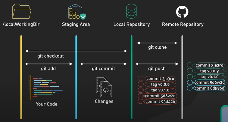
Collaboration in Git is a two-way exchange. To integrate your teammates’ work, you use git pull, which fetches changes from the remote repository and merges them into your local repository. It combines two commands: git fetch, which grabs the latest updates, and git merge, which integrates these updates with your work.
git checkout or git switch comes in. It allows you to switch between different branches to work on specific features. Git branching allows you to diverge from the main codebase to develop a new feature without impacting the main code. Some key concepts include creating a new branch with git branch, switching between branches using git switch, merging branches together with git merge, and resolving merge conflicts when changes overlap.
Branching enables isolated development and collaboration workflows. There are more nuance when merging or rebasing changes from others or managing branches.
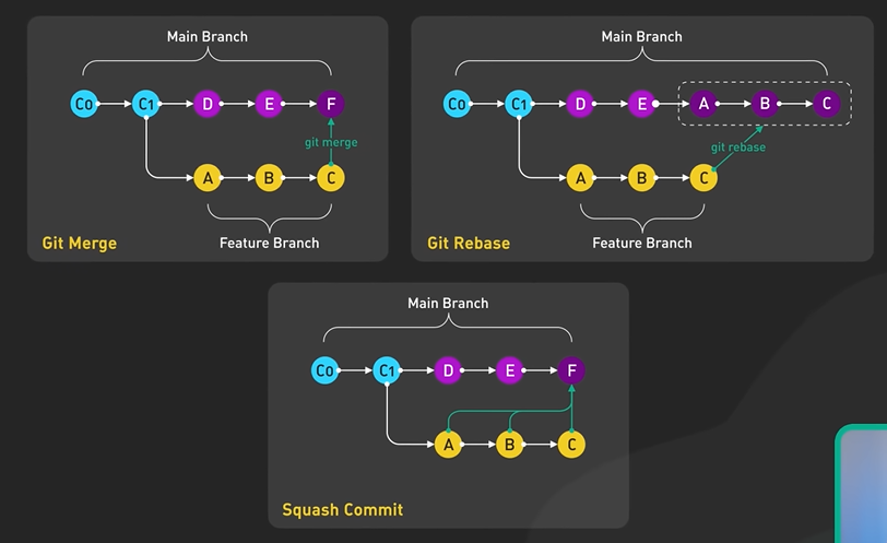
Many developers use graphical git tools like GitHub Desktop and SourceTree. These tools provide visual interfaces and shortcuts for common commands.
JWT.
https://youtu.be/P2CPd9ynFLg?si=aRmmF-D3EVDdANos
But like losing your passport, a stolen JWT gives hackers full access. In this video, we’ll unlock the immense potential of JWTs, and the dangers lurking within. I’m Sahn, co-author of best-selling system design interview books. We explain complex system design concepts clearly through animations. Let’s get started. JSON Web Tokens, commonly known as JWTs, are a robust method for securely transmitting information between parties as JSON objects. They have become a cornerstone in the world of web security for good reasons. First, let’s talk about JSON itself. It’s a lightweight data interchange format that’s easy to read and write for humans and simple for machines to parse and generate. It’s the backbone of JWTs because it represents its payload, which is where you store the data you want to transmit. Now, JWTs have a structure of three parts: the header, the payload, and the signature. Each section is base64 encoded and separated by a period. The header typically consists of the token type, which is JWT, and the algorithm being used, like HMAC SHA256 or RSA. The payload of a JWT is where you store the claims. Claims are statements about an entity, which is typically the user with some additional data. There are three types of claims: registered, public, and private. Registered claims are predefined, like the issuer, expiration time, and subject. While JWT payloads can be encrypted using JSON Web Encryption (JWE), most implementations use signed but not encrypted tokens. This means that while the data is encoded, it is not encrypted and can be read if intercepted. That’s why sensitive information should never travel in a JWT payload unless it’s encrypted first. Let’s talk about signing these tokens. Signing is like sealing an envelope with a wax stamp to ensure it hasn’t been tampered with. There are two main types of signing algorithms: Symmetric algorithms, like HMAC SHA256, use a shared secret key for both signing and verification. Asymmetric algorithms, such as RSA, use a public/private key pair where the private key signs the token and the public key verifies it. When choosing an algorithm, consider your needs. Symmetric keys are quick and simple but the secret key must be shared between parties ahead of time. Asymmetric keys allow verification of the creator without sharing private keys but are slower. Signed JWTs provide authentication, authorization, and secure information exchange. Upon login, the server creates a signed JWT with user details and sends it back. The client uses this to access protected resources by sending the token in the HTTP header. JWTs are commonly used in standards like OAuth2 and OpenID Connect for authentication and authorization. However, it’s crucial to know when not to use JWTs. The payload is not encrypted by default so should not contain highly sensitive data. Also, JWTs aren’t ideal for managing user sessions since they are stateless. Revoking JWT access can be challenging. Some common vulnerabilities to be aware of include token hijacking, where an attacker steals a valid JWT to impersonate a user. JWTs also could be vulnerable to cryptographic weaknesses if using weak hashing algorithms. Automated brute force attacks may try to crack token signatures. To mitigate risks when using JWTs, some best practices to follow are: keeping JWT payloads compact with only the necessary user claims; using short token expiration times when possible; storing tokens securely and invalidating any leaked tokens; and using strong signature algorithms . The pros are clear: JWTs are self-contained, portable, and don’t require server-side storage. On the downside, JWTs can be vulnerable to theft, and if intercepted, can provide full access to resources. The payload can also get quite large if too much information is included, which can affect performance. Overall, JWTs provide a scalable way to handle authentication, authorization, and information exchange if implemented carefully. If you like our videos, you might like our System Design newsletter, as well.
How does the Linux Boot Process work.
https://youtu.be/XpFsMB6FoOs?si=tHsaqoEGc76Kadso
What really happens behind the scenes when you press that power button to boot up Linux? Today I’ll give you an inside look. The process starts when you press that power button to turn on your computer. First, a program called the BIOS or UEFI boots up. These are basically pieces of software that get all the main parts of your computer ready for action - we’re talking about the keyboard, screen, hard drives, and so on. UEFI is the newer kid on the block, offering faster boot times and better security features like Secure Boot, compared to the traditional BIOS. One key difference between BIOS and UEFI is in their approach to disk storage. BIOS is tied to the Master Boot Record (MBR) system, which limits disk size to 2TB. UEFI, on the other hand, uses the GUID Partition Table (GPT), removing these size constraints and offering a more flexible and modern solution. BIOS UEFI BIOS is tied to the Master Boot Record (MBR) system, which limits disk size to 2TB. Slower boot time Less secure boot UEFI, on the other hand, uses the GUID Partition Table (GPT), removing these size constraints and offering a more flexible and modern solution. Faster boot time Secure boot Next, the BIOS or UEFI runs a check called the power-on self-test or POST. This test makes sure all the different hardware bits and pieces are working right before fully turning everything on. If POST finds a problem, it’ll often show an error message on the screen. Finally, if everything checks out with POST, the BIOS or UEFI needs to find and load up the boot loader software. The boot order is usually set to check the hard drive first, then USB drives or CDs if it doesn’t find anything on the hard drive. You can customize this order in the BIOS settings if you want. On a BIOS system, the boot loader code lives in the first little chunk of the hard drive called the Master Boot Record. For UEFI, there’s a separate partition that stores files like the .efi boot loader file. The key jobs for the boot loader are: Locate the operating system kernel on the disk Load the kernel into the computer’s memory Start running the kernel code Some common boot loaders you might see are LILO and GRUB2. LILO, the Linux Loader, is pretty outdated and rarely used in modern distributions. GRUB2 is the most full-featured and widely used today. It can handle booting multiple operating systems, looks nice with graphical or text-based menus, and has a bunch of advanced options for power users. So once GRUB2 loads itself up, it inserts the Linux kernel into memory and hands control over to the kernel to finish the startup process. After the boot loader starts the kernel, the kernel takes over the computer’s resources and starts initiating all the background processes and services. First it decompresses itself into memory, checks the hardware, and loads device drivers and other kernel modules. Next, an initial process called init kicks off, which in modern Linux systems is typically Systemd. Systemd has replaced older init systems like SysVinit and Upstart and is the parent of all other processes on Linux. Systemd has a ton of responsibilities to get the system booted and ready to use. It’s checking for any remaining hardware that needs drivers loaded. It mounts up all your different file systems and disks so they’re accessible. It starts launching all the background services you need like networking, sound, power management. It handles user logins once you get to the graphical prompt. And it loads up your desktop environment with the panels and menus. Systemd uses target configuration files to decide which mode it should be booting into - something basic like multi-user text-only target, or the graphical target most of us use daily. Those targets kind of correspond to the old run levels from past Linux days if you’ve heard of those. Mostly now you just need to know Systemd handles initializing everything that needs to launch behind the scenes when starting up Linux.
Vertical vs Horizontal Scaling.
Vertical scaling means adding more power to your existing server. This could involve adding more CPUs, RAM, storage, or network bandwidth.
Horizontal scaling means adding more servers to your infrastructure and distributing the workload across them. This is also known as “scaling out.”
High availability. Lower cost over time. Improved performance.
Most popular type of API testing.
There are 9 types of API Testing -
Smoke Testing.
Functional Testing.
Integration Testing.
Regression Testing.
Load Testing.
Stress Testing.
Security TEsting.
UI testing.
Fuzz Testing.
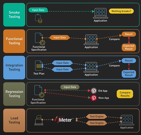
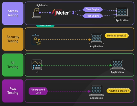
Smoke Testing is like a quick test drive for APIs. We run basic tests to confirm the API is working and responding to simple requests.
Functional Testing does the same for APIs. We create detailed test cases to ensure all functionalities of the API are working as expected and meet specific requirements. These functional test suites ensure features like product search, adding items to a cart, and secure checkout are all working. Large-scale systems can involve many different APIs working together seamlessly.
Integration testing ensures these diverse APIs and cloud services communicate and exchange data correctly. For example, for a travel booking website, integration testing verifies that the airline reservation API properly coordinates with payment, passenger identity, and other systems behind the scenes. And of course, new updates and code changes can inadvertently introduce problems.
Regression testing replays existing test cases against updated versions of the API to check for defects or regressions. This allows developers to iterate without worrying about collateral damage - no taking one step forward and two steps back.


Load testing evaluates real-world performance by bombarding the API with high user volumes.
Stress testing takes this to the extreme, simulating drastic traffic spikes and edge conditions way beyond normal usage. Both prepare APIs to maintain responsiveness and stability during crunch times, whether it’s the holiday e-commerce rush or a viral social media hit.
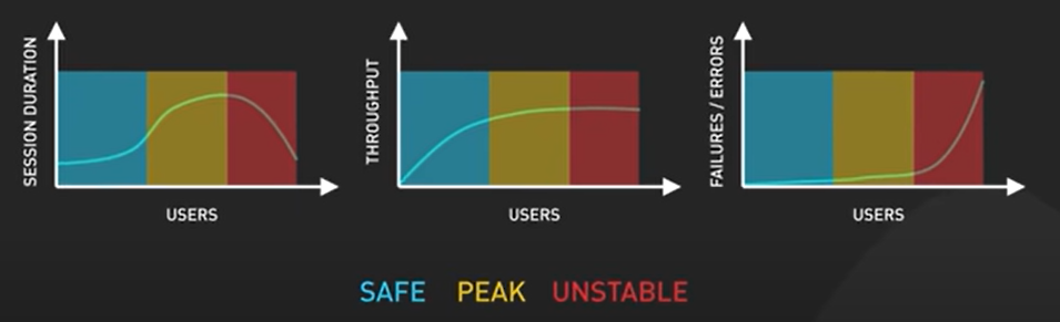
Security is very important, as APIs access sensitive systems and data. Security testing probes APIs for any weaknesses or loopholes that could allow unauthorized access or cyber threats.
Proactively addressing vulnerabilities fortifies APIs against attacks to keep customer data safe, just like a bank vault protects valuables.
UI Testing ensures APIs contribute to a seamless user experience. Fast response times during map rendering and navigation in ride-sharing apps for example directly correlate to positive UI perceptions.
Fuzz testing takes it one step further by deliberately throwing malformed, unexpected, or randomly generated data at APIs to identify edge cases. Subjecting systems to unusual data volumes and formats hardens them against unpredictable real-world usage down the line.
Client Architecture Pattern.
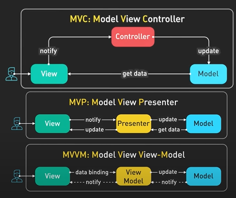
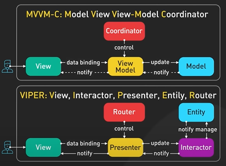
The MVC, or Model-View-Controller pattern, is almost half a century old! It was a groundbreaking approach that separated UI, data, and control logic to allow developers to focus on these pieces individually.
It is a simple flow but can lead to a bloated controller when the app grows.
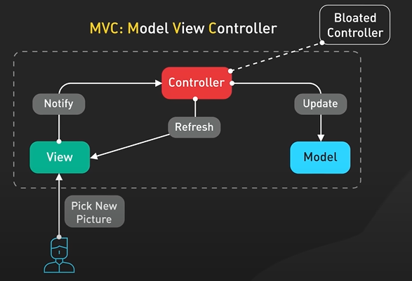
MVP introduces a more prominent Presenter that handles UI logic - transforming model data for display, handling user inputs, and coordinating model and view updates.
By isolating UI logic, MVP enables the View to focus strictly on drawing visuals for cleaner code and testing.
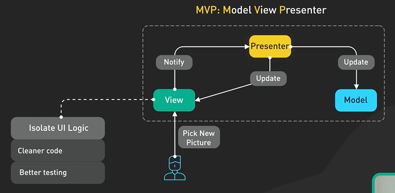
MVVM introduces data binding between the View and ViewModel. It enables automatic propagation of data changes in both directions. It reduces the need for explicit update logic.
The ViewModel handles syncing raw Model data to reflect UI changes automatically. The ViewModel persists this change to the Model. Any Model data updates automatically reflect back on the bound View properties without needing explicit refresh calls.
By handling bi-directional syncing between View and Model, data binding streamlines updates that would otherwise require boilerplate code.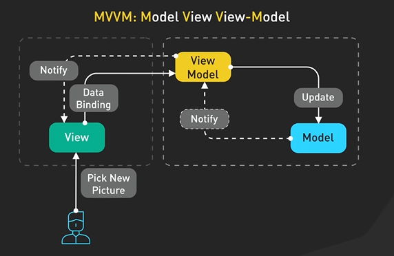
MVVM-C goes further by adding a Coordinator layer to oversee navigation logic. Building on top of MVVM data binding, the Coordinator centralizes flow control needed for transitions between screens and use cases. In our example, this means moving from the profile screen to image selection, then back again, while managing saving logic. This responsibility is handled by the Controller rather than the ViewModel. It allows the ViewModel to focus solely on data handling.
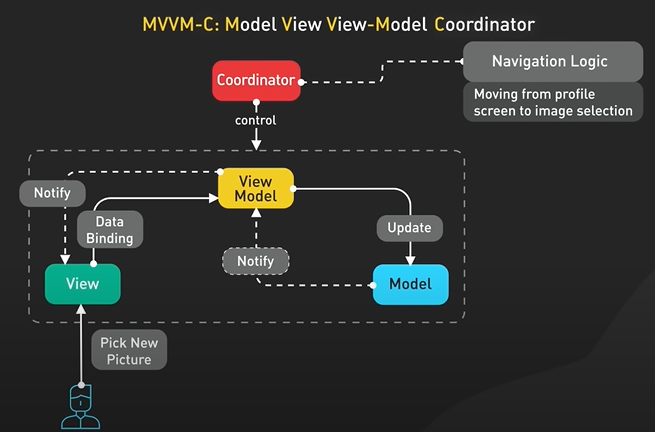
The View only displays the user’s action, the Interactor handles the business logic of the image update, the Presenter updates both the View and the Entity which is the Model equivalent, and the Router manages the navigation. This modular approach is especially powerful for large, complex applications.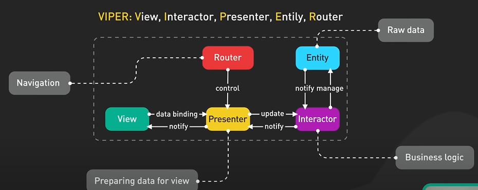
So, which pattern should you choose?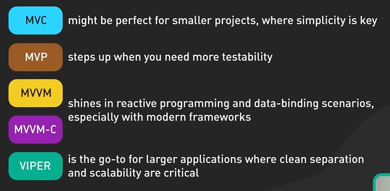
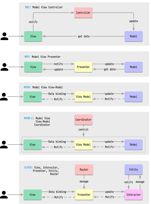
Linux File System Explained.
Have you ever wondered how Linux organizes all its folders and files behind the scenes? In the early days, it was pure chaos, with every distribution implementing its own structure. I still remember the first time I tried finding a config file in RedHat Linux - I was totally lost. To create order from the chaos, the Linux community rallied around the Filesystem Hierarchy Standard (FHS). This established a consistent directory structure so users could find what they needed on any distribution. But does every distro follow it exactly? Not always! Some add custom tweaks for their specific needs. Understanding where critical system files, configurations, and binaries live allows us to navigate any Linux environment and harness its full power. Let’s explore the key directories at the heart of the Linux file system. First, the homes for executable binaries. The layout of directories like /bin, /usr/bin, /usr/local/bin and their sbin counterparts follows a convention. /bin contains core OS programs that must be accessible before /usr gets mounted at boot. For example, the commands mount, ls, cd live here. /usr/bin is a primary home for binaries NOT part of the base OS itself. Most user programs live here. Fun fact: usr stands for Unix System Resources, not user! /usr/local/bin holds executables installed by the admin, usually after building them from source. This keeps local compiles separate to avoid overwriting system binaries. The sbin directories follow a similar pattern but house sysadmin utilities that require root access like iptables and sshd. When the same binary exists in multiple directories, you can specify the default by reordering the directory precedence in the PATH variable. /lib contains shared library files essential for /bin and /sbin binaries to function properly. These libraries need to be accessible early in the boot process before mounting /usr. They provide core functionality like C library routines (glibc) and compiler runtimes (libstdc++). /usr/lib holds libraries for /usr binaries that aren’t critical for early system initialization. This includes UI libraries like GTK and Qt as well as language runtimes like Python. You can also tweak the library search order via LD_LIBRARY_PATH. Now onto /etc - the home of Linux configuration files! Text-based config files here control everything from networking to authentication services. Ever scratched your head when digging through fstab and ssh_config? I certainly have! For user data, /home stores documents, media and projects while administrators have the exclusive /root folder. Fast-changing data like logs and caches live under /var. It is always buzzing with activity. We care about /var/log in particular to inspect hardware events, security issues, or performance problems. /run contains volatile run-time info like systemd details, user sessions and logging daemons. System services use /run for ongoing communication via sockets and lock files. For example, mysql.sock might be crucial for database access. Finally, we come to the interconnected /proc and /sys virtual filesystems for Linux experts. /proc opens communication channels to inspect overall OS state - we can check high-level metrics via cpuinfo, view filesystem mounts, and dive deeper with tools like lsof, strace, and pmap. /sys exposes lower-level kernel and hardware objects, allowing granular monitoring and configuration of components like devices, modules, network stack via virtual files. Combined, they provide complete system observability spanning high level metrics to low level component interactions. With /proc oriented towards process/runtime statistics and /sys providing component/hardware access, these inspection points are useful for performance tuning and forensic triage. You now have a roadmap to freely access critical Linux filesystem resources. Armed with this knowledge, you’re ready to take full command. How about we get some hands-on practice?
How Disney captures 1B emojis.
https://youtu.be/UN1kW5AHid4?si=v14PZ9zyoXBMWRU1
Today, we’re plunging into how Disney Hotstar aced the extraordinary challenge of managing 5 billion emoji reactions during a high-tension Cricket World Cup match. Image this. A thrilling match had millions of fans glued to their screens. As excitement built up, millions of emotional fans flooded Hotstar’s backend with emoji reactions, pushing their servers to the limit. Let’s explore how Hotstar solved this difficult engineering challenge and turned passive viewers into an active community united by the rollercoaster of emotions that only live sports can stir up. First solution? An architecture hinges on asynchronous processing across decoupled components. This approach is critical for scale, speed, and resilience under extreme loads. Ingestion is handled by Kafka, an open-source distributed event streaming platform. Kafka uses topics to organize data streams and consumer groups to enable parallel processing. This capacity to buffer huge streams of data from multiple sources made it an ideal choice to handle the high volumes of emojis. The client apps transmit emoji reactions to API servers built with Golang, an open-source programming language developed by Google. The lightweight Goroutines enable massive concurrency while Go’s channels provide inter-process communication to exchange data safely between Goroutines. Together, these primitives allow Hotstar’s APIs to accept incoming reactions from millions of viewers, batching them using channels, and asynchronously write the events to Kafka topics in batches. This setup allows Hotstar to efficiently handle millions of concurrent emoji reactions without overwhelming the servers. Next, Spark, a fast unified analytics engine built on the JVM, processes this torrent of emoji stream from Kafka, updating sentiment scores every 2 seconds to reflect changing audience moods in real-time. By leveraging in-memory processing, Spark can run certain workloads 100x faster than previous disk-based big data platforms like Hadoop MapReduce. Spark Streaming’s micro-batch architecture is crucial here. It allows Hotstar to process data in small, manageable chunks. Instead of processing each reaction individually as it arrives, Streaming divides the continuous data flow into small time-sliced batches. Spark then runs aggregation algorithms on the batched streaming data to determine emoji sentiment distributions across users, visualizing dynamic shifts in audience reactions. The aggregated sentiment data is routed into a separate Kafka topic that buffers it before final delivery. A Python consumer pulls from this Kafka topic and publishes the sentiment data to Hotstar’s PubSub messaging infrastructure. This custom-built PubSub messaging system is the final piece of the whole setup. It quickly sends sentiment data to millions of devices. Built on MQTT, it’s designed to handle large amounts of content while keeping delays low. It plays a critical role in making sure that the audience gets real-time updates without any hiccups. To wrap it up, Hotstar’s decoupled architecture enables each component to scale independently. It ensures smooth streaming during one of the most intense sports events, proving that smart engineering can turn even the heaviest data loads into a seamless experience for millions. The results speak for themselves. Latency dramatically reduced from 6 seconds to a mere 2 seconds. System outages are a thing of the past, and there’s an 85% reduction in costs.
Tips for API design.
Use Clear Naming.
/carts - Collection of carts.
/products - Collection of products.
Ensure reliability through idempotent API.
Put is idempotent and it update the data.
Patch update the selected part of the data and it is not idempotent. Like update an array and add value to it and again use the patch command it will again add the value.
Add versioning.
v1/carts/123 and used like v2/carts/123.
Versioning allow the backward compatibility.
Add pagination.
Page offset and cursor based.
Page offset pagination uses number based record like page 2 will contain record 11 to 20 and size 10.
Cursor-based pagination takes a pointer and return the next record.
Use clear query strings for sorting and filtering API data.
Sort the data by registered the Url can be GET/users?sort_by=registered
Only need color product - GET/products?filter=color:blue
User can see the active filters. Additional search and filter can be added without breaking any existing condition.
Security of the API.
Keep cross resource references simple.
Use clear linking between connected resources.
Reference item 321 in the cart 123 should be like this carts/123/items/321 and not items?card_id=123&item_id=321
Plan for rate limiting.
It protects api from over use. There should be a validation in the source ip address, endpoint and user account. Free user should make 1000 calls and one ip can make 20 calls in a specific time.
Diagram as Code.
https://youtu.be/jCd6XfWLZsg?si=H95NOyWcxcLzsgxI
Today I’m showcasing six cool tools that convert code into architectural diagrams. Whether you’re a developer documenting systems or a tech lead sharing knowledge, I think you’ll see some awesome options here. First up is Diagrams - a Python library that lets you draw cloud system architectures in code. It was created for rapidly prototyping new designs without separate diagramming tools. Representing diagrams as code allows tracking of diagram changes in version control systems. This “diagram as code” approach bridges documentation with system implementation. Diagrams supports visualizing infrastructure across major providers and stacks: AWS, Azure, GCP, Kubernetes, and more. It can also model on-premise nodes, SaaS services, and major programming frameworks and languages. The extensive catalog of icons and intuitive syntax accelerates diagram creation for modern tech stacks. If you prefer Go, there is Go-Diagrams. It’s the same idea as the python version, but let’s you write in Go. Next is Mermaid - it enables creating diagrams and visualizations using text. As a JavaScript library, Mermaid uses Markdown-style text definitions that feed into a renderer to modify complex diagrams. Their stated goal is to help documentation keep pace with development. Mermaid aims to solve “doc-rot” - where diagramming and docs take precious developer time yet still get outdated quickly. This ruins productivity and organizational learning. Mermaid enables even non-programmers to create detailed visuals through the Mermaid Live Editor. If you want an even more powerful diagramming tool, check out PlantUML. It offers a domain-specific language to generate many diagram types: sequence diagrams, architectural diagrams, network topology, Gantt charts, and even ASCII art. PlantUML’s language is very capable but has a bit more learning curve compared to other tools we covered. The broad features make PlantUML a flexible, powerful option for embedding diagrams alongside code. The next category of tools goes in the opposite direction - ASCII diagram editors. These tools allow you to draw diagrams visually or in text and then render them as ASCII art. They harness the power and simplicity of plain text, which has been around for decades. ASCII editors let you easily author text-based diagrams, layouts, flow charts, and more. Since they output in plain text format, these diagrams can embed anywhere. Some examples of this class of tools include web-based asciiflow and Monodraw, which is Mac only. Finally, Markmap creates and visualizes mind maps derived from Markdown documents. It parses Markdown content and extracts its inherent hierarchies to render a mindmap. It’s great for connecting ideas and their relationships defined in writing. It supports various platforms but may not work well on very large or complex mind maps. if you like our videos, you might like our System Design Newsletter as well. It covers topics in trends and large-scale system design. Trusted by 500,000 readers. Subscribe it at blog.bytebytego.com.
Webhooks.
https://youtu.be/x_jjhcDrISk?si=veNNKiZd3gmH7tEK
Today, we’re diving into the world of webhooks and how they stack up against old-school methods like long and short polling. If you’ve ever run an eCommerce website or dealt with APIs, you’ll want to stick around for this. Imagine you have an eCommerce site. Your customers are happily clicking away, adding items to their carts, and hitting that sweet ‘Order’ button. Their requests zip through the API gateway and land at the Order Service, which then passes the baton to the Payment Service to handle the transactions. This is where our external Payment Service Provider, or PSP for short, comes into play—let’s call our PSP “Stripe.” So, how does Stripe communicate with your website to confirm that the payment is good to go? Traditionally, we’d use what’s called ‘short polling’. It’s like repeatedly asking, “Are we there yet?” on a long car ride. After sending the payment request to Stripe, your Payment Service would keep checking in: “Is the payment ready? How about now?” And this would go on until Stripe finally says, “Yep, all good here!” But, hold on, there’s a catch. Short polling is like a needy app that’s always asking for updates. It can be a bit of a resource hog. What about long polling? Think of long polling as a more patient sibling of short polling. Instead of constantly asking for updates, the server holds the request open for a while and only responds when there’s new information. It’s better, but still not perfect. You’re waiting on the line, and it can be tough on server resources. Enter webhooks. Instead of bugging Stripe for updates, you simply say, “Hey, hit me up at this URL when you’ve got news.” Once Stripe processes the payment, it makes a beeline to your specified URL to drop off the status update. No more wasted resources and constant nagging. You might hear folks call webhooks reverse APIs or push APIs since the server is reaching out to the client with info, not the other way around. But to keep things running smoothly, here are some best practices to follow. One: Have a fallback polling mechanism in place to detect failed deliveries. Things happen, servers go down. So having a periodic poll as a backup ensures you don’t miss critical updates. In our example, what if Stripe forgets to call? Have a housekeeping job that checks in every so often, just to make sure everything’s on track. Two: Secure webhooks with secrets and tokens. You don’t want just anyone calling your webhook endpoint. Requiring authentication tokens helps prevent abuse. Verify each call’s signature to ensure it’s really Stripe on the line, not an impostor. Three: Make webhook idempotent. That means code defensively so if a webhook is delivered more than once, it doesn’t cause issues. Include unique identifiers to de-dupe where possible. Four: Watch out for webhook overload. If you suddenly get popular, can your infrastructure handle a surge in webhook traffic? Plan ahead. For high-volume websites, use queues to decouple the receiving and processing of webhook events. When your site goes viral, you’re ready for the spotlight. And webhooks may not be the answer when real-time data with microsecond latency is absolutely essential. For the most time-sensitive applications, a persistent socket connection enables push updates with lower overhead than webhooks but is more difficult to set up and scale. However, the performance is better. There are definitely tradeoffs to consider, but webhooks unlock big efficiency gains when applied properly. If you like our videos, you might like our system design newsletter as well. It cover topics in trends and large-scale system design. Trusted by 500,000 readers. Subscribe at blog.bytebytego.com.
Caching pitfalls.
https://youtu.be/wh98s0XhMmQ?si=qOxkUDq7qeMpXHpR
Today we’re going to talk about caching - a key concept in system design that is critical for performance but can also cause some issues if not handled properly. Before jumping into what can go wrong, let’s quickly cover the basics of what caching is and why it matters. Simply put, caching is like a memory layer that stores copies of frequently accessed data. It’s a strategy to speed things up by keeping data readily available, reducing the need to fetch it from slower databases every time it’s requested. For example, think about a database with user profiles. A cache for this database might store the most popular user profiles so that when someone views a profile, it loads instantly instead of hitting the database on every view. Now even with these performance gains, caching also introduces new challenges. Let’s unpack the common problems that can come up. First up, let’s explore Cache Stampede. Imagine a web server using Redis to cache pages for a set duration. These pages require extensive database calls and take several seconds to render. With caching, the system stays responsive under high load since resource-heavy pages are served from cache. However, under extreme traffic, if a cached page expires, multiple threads across the web cluster may try refreshing the expired page at the same time. This flood of requests could overwhelm the databases, potentially causing system failure and preventing the page from being re-cached. So how can we prevent stampedes? A few key strategies: One is locking. Upon a cache miss, each request attempts to acquire a lock for that cache key before recomputing the expired page. If the lock is not acquired, there are some options: One, the request can wait until the value is recomputed by another thread. Two, the request can immediately return a “not found” response and let the client handle the situation with a back-off retry. Three, the system can maintain a stale version of the cached item to be used temporarily while the new value is recomputed. Locking requires an additional write operation for the lock itself, and implementing lock acquisition correctly can be challenging. Another solution is offloading recomputation to an external process. This method can be activated in various ways - either proactively when a cache key is nearing expiration, or reactively when a cache miss occurs. This approach adds another moving part to the architecture that requires careful ongoing maintenance and monitoring. A third approach is probabilistic early expiration. In this strategy, each request has a small chance of proactively triggering recomputation of the cache value before its actual expiration. The likelihood of this happening increases as the expiration time approaches. This staggered early refreshing mitigates the impact of the stampede since fewer processes will expire. Moving on to Cache Penetration. This happens when a request is made for data that doesn’t exist in the cache or the database or cache. This results in unnecessary load, as the system tries to retrieve non-existent data. This can destabilize the entire system if the request volume is high. To mitigate cache penetration, implement a placeholder value for non-existent keys. This way, follow-up requests for the same missing data hit the placeholders in cache instead of pointlessly hitting the database again. Setting appropriate TTL for these placeholders prevents them from occupying cache space indefinitely. However, this approach requires careful tuning to avoid significant cache resource consumption, especially for systems with many lookups of non-existent keys. Another approach uses bloom filters, a space-efficient probabilistic data structure for quickly checking if elements are in a set before querying the databases. Here’s how they work: when new records are added to storage, their keys are recorded in the bloom filter. Before fetching records, the application checks the bloom filter first. If the key is absent, the record conclusively doesn’t exist, allowing the application to return a null value immediately. However, positive key presence doesn’t guarantee existence - a small percentage of cache reads may still result in misses. We have a video on how bloom filters work if you want to learn more. Finally, we come to the Cache Crash. Picture this: our entire cache system suddenly fails. What happens next? With no cache layer, every single request now slams straight into the database. This sudden spike in traffic can easily overwhelm databases, jeopardizing overall system stability. What’s worse? Users start obsessively hitting refresh, compounding the problem. A close cousin to the Cache Crash is the Cache Avalanche. This can happen in two scenarios. One, when a massive chunk of cached data expires all at once. Two, when the cache restarts and it is cold and empty. In both cases, a crushing wave of requests hits the databases all at once. This sudden load spike overwhelms the system, much like hundreds of people abruptly cramming through a single tiny door after a fire alarm. So how do we tackle these challenges? First option: implement a circuit breaker, which temporarily blocks incoming requests when the system is clearly overloaded. This prevents total meltdown and buys time for recovery. Next strategy, deploy highly available cache clusters with redundancy. If parts of the cache go down, other parts remain operational. The goal is to reduce the severity of full crashes. And don’t dismiss cache prewarming. Particularly critical after a cold start. Here, essential data is proactively populated in the cold cache before it’s put into service. This avoids abruptly bombarding the databases. As we wrap up, let’s distinguish cache stampedes versus cache avalanche since they sound similar. A cache stampede happens when many requests simultaneously hit the same expired cache entry, overwhelming the database as it tries to refresh just that single data point. The cache avalanche is a broader issue where numerous requests for different data flood the system after a cache is cleared or restarted, putting a strain on resources. And that concludes our walkthrough of the common caching pitfalls and how to navigate them. If you like our videos, you may like our system design newsletter as well. It covers topics and trends in large-scale system design. Trusted by 500,000 readers. Subscribe at blog.bytebytego.com.
Reverse Proxy API Gateway Load Balancer.
https://youtu.be/RqfaTIWc3LQ?si=BfKR8uMmBIRl6AV-
Why Kafka is popular.
https://youtu.be/yIAcHMJzqJc?si=tqlNEjxXKM6ZsUKM
In this video, we’re exploring the top five use cases for Apache Kafka. As a distributed event streaming platform, Kafka has revolutionized the way companies handle real-time data. These popular use cases showcase Kafka’s power in handling real-time data streams. First on our list is log processing and analysis. Kafka’s ability to handle massive volumes of log data makes it an ideal choice for this use case. Imagine a complex microservices architecture where multiple services, such as the Shopping Cart, Order Service, and Payment Service, generate a massive amount of log data. Kafka acts as a centralized log aggregation system, ingesting and storing these logs at scale. It provides a short-term durable storage layer for log data, retaining logs for a configurable retention period, typically in days. This allows organizations to centralize their logging infrastructure. Kafka integrates seamlessly with the ELK stack, providing powerful log analysis and visualization capabilities. Next, let’s talk about data streaming for recommendations. Picture a world where every recommendation feels like it’s made just for you. Kafka makes this a reality by powering real-time data streaming pipelines for recommendation engines. It processes user click streams and aggregates data in a Data Lake for deep analysis. Flink, a powerful stream processing framework, can be used with Kafka to perform real-time analytics and machine learning on the streaming data. This allows for the continuous improvement of recommendation accuracy based on up-to-date user behavior. With Kafka’s low-latency streaming capabilities, users receive real-time, personalized recommendations that enhance their experience. The third use case is system monitoring and alerting. With today’s ever-growing system complexity, proactively detecting and resolving issues is essential. Kafka ingests metrics and events from various services, enabling fast detection of anomalies or critical events. Organizations can use stream processing tools like Flink to define alerting rules and thresholds based on real-time data. When an issue is detected, alerts are triggered and sent to the relevant teams, enabling prompt action and quick resolution. Kafka’s ability to process high-velocity data streams makes it a great platform for building real-time monitoring and alerting systems. Moving on to the fourth use case, we have Change Data Capture, or CDC. Imagine the challenge of keeping data in sync across multiple databases and applications. Kafka comes to the rescue by capturing changes made to source databases, such as transaction logs, in real time. With the help of Connectors like the ElasticSearch Connector and Redis Connector, Kafka propagates these changes to target systems reliably. CDC ensures data consistency and synchronization, reducing discrepancies and enabling real-time data integration. Kafka’s flexibility supports various databases, making it a good tool for CDC implementations in diverse environments. Finally, let’s discuss system migration. Upgrading or migrating systems can be a daunting task, but Kafka makes it less painful. Kafka acts as a data bridge between the old and new versions of services during system migration. Let’s consider a scenario where an organization is migrating their services on V1 to V2. Kafka ensures data consistency and availability throughout the migration process by replicating data between the old and new versions of each service. This allows for a seamless transition without any data loss or disruption to the overall system. Kafka’s ability to decouple systems allows for a phased migration approach, reducing risks and minimizing downtime. Pre-migration reconciliation can be performed by comparing results from the old and new versions, ensuring data integrity every step of the way. Apache Kafka is a versatile and powerful tool that enables organizations to handle real-time data effectively across various use cases. Consider Kafka for your next data-intensive project. If you like our videos, you may like our system design newsletter as well. It covers topics and trends on large-scale system design. Trusted by 500,000 readers. Subscribe at blog.bytebytego.com.
ACID properties in DB.
https://youtu.be/GAe5oB742dw?si=6MJdW1g2UOF0BxDh
ACID stands for Atomicity, Consistency, Isolation, and Durability - the four key properties that ensure reliable database transactions, even when things go wrong. If you work with databases, understanding ACID is a must. In this video, we’ll break down each property and see how they keep the data safe and sound. Let’s dive in! Atomicity means a transaction is an all-or-nothing deal. If any part of the transaction fails, the whole thing gets rolled back like it never happened. Transaction management systems often use logging mechanisms to enable this rollback feature. Imagine you’re building a banking app that transfers $100 from Alice to Bob. This means updating two things - subtracting $100 from Alice’s balance and adding $100 to Bob’s. Atomicity ensures that both updates either happen together or not at all. If something fails midway, the transaction management system will use the logs to undo any partial changes, so you won’t end up with lost or extra money. The transaction is indivisible, like an atom. Consistency means that a transaction must follow all the rules and leave the database in a good state. Any data written during a transaction must be valid according to constraints, triggers, and other rules we’ve set up. The database system itself enforces consistency by automatically checking for constraint violations during transactions. For example, let’s say we have a rule that user account balances can’t go negative. If a transaction tries to withdraw more money than a user has, the database system will detect this consistency violation and cancel the transaction to keep the database consistent. Consistency stops invalid data from messing up the database. Isolation is all about how concurrent transactions interact with each other. Even if many transactions are running at the same time, isolation makes it seem like each transaction has the database all to itself. The highest level of isolation is called “serializable.” It makes transactions run one after another as if they were in a single line. This provides the strongest consistency, but it can really slow things down because each transaction has to wait its turn. To speed things up, databases often provide lower isolation levels that allow more transactions to run simultaneously. But there’s a catch - these lower levels can sometimes lead to inconsistencies, like dirty reads, non-repeatable reads, and phantom reads. A dirty read happens when a transaction sees data that was changed by another transaction that hasn’t been committed yet. Imagine a bank account with $100. Transaction T1 withdraws $20 but doesn’t commit. If Transaction T2 reads the balance before T1 commits, it will see $80. But if T1 rolls back, that $80 balance never truly existed - it’s a dirty read. The “read committed” isolation level prevents dirty reads by making sure a transaction can only see committed data. But it can still have non-repeatable reads, where a transaction reads the same data twice and gets different results because another transaction changed the data in between. For example, say you check your bank balance and see $100. Then another transaction withdraws $20 and commits. If you check your balance again in the same transaction, you’ll see $80. That’s a non-repeatable read. “Read committed” can also have phantom reads, where a transaction re-runs a query and gets different results because another transaction added or deleted rows that match the search criteria. Imagine a transaction that lists all bank transfers under $100. Meanwhile, another transaction adds a $50 transfer and commits. If the first transaction reruns its query, it will see the $50 transfer that wasn’t there before - a phantom read. The “repeatable read” isolation level prevents non-repeatable reads by giving each transaction a consistent snapshot of the data. But it can still have phantom reads. So, lower isolation levels trade some consistency for better performance. It’s up to you to choose the right balance for your application, weighing speed against potential inconsistencies. Durability means that once a transaction is committed, it’s permanent - even if your database crashes or loses power right after. Durability is usually achieved by writing transaction logs or using write-ahead logging (WAL) to persist changes to disk before confirming the commit. In distributed databases, durability also means replicating data across multiple nodes. So if one node goes down, you don’t lose any committed transactions - they’re safely stored on the other nodes. To quickly sum up - Atomicity rolls back failed transactions, Consistency follows the rules, Isolation prevents interference, and Durability makes sure commits stick. If your like our videos, you might like our system design newsletter as well. It covers topics and trends in large-scale system design. Trusted by 500,000 readers. Subscribe at blog.bytebytego.com.
Learning SQL.
https://youtu.be/yMqldbY2AAg?si=tJjtmKTDxCWx6LwH
SQL, or Structured Query Language, is the standard language for interacting with relational databases. Its versatility makes it an essential tool across industries. For example, an e-commerce company might use SQL to analyze sales data, identify trends, and make data-driven decisions to optimize its business strategy. Popular relational database management systems that use SQL include MySQL, PostgreSQL, Oracle, and SQL Server. In this video, we’ll explore the key concepts and techniques you need to know to work effectively with SQL. At the core of SQL are databases, which store and organize data. Within a database, data is structured into tables, with columns defining data fields and rows representing individual records. Effective database design involves normalization, a process of organizing data to minimize redundancy and dependency. To maintain data integrity, tables utilize constraints. Primary keys uniquely identify each row, while foreign keys establish relationships between tables. For instance, a “products” table might have a primary key, “product_id,” and an “orders” table could use “product_id” as a foreign key to link each order to a specific product. Other constraints include UNIQUE, which ensures no duplicate values; CHECK, which enforces conditions on data; and DEFAULT, which specifies a default value for a column. SQL provides a range of operations to interact with data. The SELECT statement retrieves data from one or more tables, allowing filtering, sorting, and joining. JOIN operations combine data from related tables, with different types like INNER JOIN, LEFT JOIN, RIGHT JOIN, and FULL OUTER JOIN. For example, an INNER JOIN on the “customers” and “orders” tables would return all customers with their associated orders, excluding customers without orders and orders without a customer. To manipulate data, we use INSERT to add new records, UPDATE to modify existing data and DELETE to remove records. These operations can be combined with subqueries, which are nested queries within another SQL statement. For instance, you could use a subquery in an UPDATE statement to change values based on conditions from another table. SQL supports various operators and functions for filtering and transforming data. Logical operators (AND, OR, NOT) allow compound filter conditions, while numeric operators handle arithmetic operations. String operators enable pattern matching and concatenation. Functions offer powerful data analysis and manipulation capabilities. Numeric functions perform calculations like SUM, AVG, and ROUND. String functions manipulate text, such as CONCAT for combining strings or SUBSTRING for extracting characters. Date and time functions handle operations on temporal data, like GETDATE for the current date/time or DATEADD for modifying dates. Aggregate functions (COUNT, MIN, MAX, etc.) summarize data across multiple rows. T hey are often used with GROUP BY and HAVING clauses for advanced analysis. For example, you could use COUNT and GROUP BY to get the number of orders per customer and HAVING to filter only customers with more than 10 orders. When creating tables, columns are defined with specific data types to optimize storage and performance. Key types include numeric (INT, DECIMAL), string (VARCHAR, TEXT), date/time (DATE, TIMESTAMP), and boolean (BIT). Indexes are crucial for optimizing query performance, especially on large tables. Indexes allow faster queries by creating a searchable structure, similar to an index in a book. However, they also introduce overhead for insert, update, and delete operations. Beyond data manipulation (DML), SQL includes sub-languages for other tasks. The data definition language (DDL) handles table structure with statements like CREATE TABLE and ALTER TABLE. The data control language (DCL) manages access permissions using GRANT and REVOKE. The transaction control language (TCL) handles transaction management with COMMIT, ROLLBACK, and SAVEPOINT, ensuring data integrity through ACID properties. SQL is a powerful language for working with relational databases. The best way to learn is through hands-on practice with real-world datasets. Explore SQL tutorials and online practice platforms, and experiment with sample databases. As you advance, dive into topics like query optimization, database normalization, and transaction management. With SQL in your toolkit, you’ll be equipped to tackle complex data challenges and drive data-informed decision-making in your projects.
API Security.
https://youtu.be/6WZ6S-qmtqY?si=_Ho0QeMk5n69tWWm
Blogs for Engineers.
https://youtu.be/UuT61kf292A?si=MenqyV_LFeMHCpGN
today we’re going to explore some of the best engineering blocks out there these blocks are the go M of information offering insight into how some of the biggest tech companies tackle their engineering challenges so let’s dive in and take a look at our top n favorites first up is the Netflix Tech blog Netflix is known for its extensive use of cloud computing the blog covers a wide range of topics from microservices to data pipelines his most famous series of blog post is about his chaos monkey tool chaos monkey is a part of a suite of tools designed to test and improve the resilience of Netflix Cloud infrastructure it works by intentionally disabling instances in production to ensure that the system can withstand failures without significant customer impact the blog post highlights Netflix commitment to maintaining system resilience through continuous testing and Improvement of its infrastructure next we have the Uber block Uber has revolutionized the transportation industry and it blogs give us a peak into the engineering behind it a popular post highlights how Uber uses machine learning and AI to tackle challenges such as forecasting demand modeling and dynamic pricing Uber applies ml to optimizes realtime dispatch system efficiently matching riders with nearby drivers Uber demonstrates how Cutting Edge Technologies can solve real world problems and transform industries by harnessing machine learning and AI the cloud flare block is another mustre as a leading provider of CDN and dos Protection Services Cloud Flare’s blog offers deep insights into keeping website fast and secure the incredible depth and breath of topics is hard to pick a favorite one classic post how to receive a million packets per second dives into the challenges of achieving High packet processing rates on Linux systems it explores using multiq Nix to distribute the load across CPU course it explains how Nicks work in incredible depth moving on we have engineering at meta as one of the largest social network in the world Met has some serious engineering challenges their blog covers everything from scaling their databases to using AI to detect fake news one SEL post focuses on Rox DB an embeddable persistent key Value Store designed for fast storage Rox DB’s plugable architecture allows for customization and optimiz ation enabling matter to handle pedabytes of data and power real time user facing products for their massive user base the post highlights Rock DB’s adaptability such as implementing key exploration using compaction filters which help meta tackle unique challenges and scale the infrastructure effectively LinkedIn engineering is another great resource LinkedIn is the world largest Professional Network and its blog offers a behind the scene look at how it builds and scale it platform the most memorable blog post announces the birth of Kafka and discusses the critical role of logs in distributed Data Systems and realtime application architectures logs are foundational to understanding various software systems including databases no SQL stores replication mechanisms and Version Control Systems the article helps popularize the concept of logs among software Engineers the Discord blog is a hidden Jam Discord is a popular chat app for gamers but it blogs is relevant to anyone interested in system design it has a series of great posts about how it uses Elixir to build highly concurrent systems as an early adopter Elixir Discord leveraged the erling VM to handle millions of events per second and support millions of concurrent users however scaling system presented challenges the blog posts detail the lessons learn and libraries created throughout this course journey to make Alexa work effectively for the growing platform AWS architecture is a mustre for anyone using Amazon web services AWS is the largest cloud provider in the world and its blog is full of case studies and best practices for using its services for example the L architect series focuses on cloud architecture best practices and various architectural patterns that can be implemented using AWS Services the series includes case studies tutorials and Technical deep Dives that help readers apply the well architector framework principles to real wellth scenarios select engineering is another block worth checking out as a popular chat app for businesses select blocks offers insights into how it builds and scales its platform to handle a high volume of data and user traffic one great post discusses how slack uses retest a tool that sits on top of MySQL to facilitate easier horizontal scaling and manage shorting select system is real heavy requiring optimization strategies like archiving older messages and implementing a rep application factor of three for durability and Disaster Recovery finally we have the stripe block stripe a payment processing company offers insight into building reliable and secure Financial systems one of its most popular posts discusses how stripe uses machine learning to detect fraud in real time through a strip radar solution strip radar accesses the risk of forent transactions in less than 100 milliseconds the blog post details radar Evolution over nearly 7 years highlight improvements in this machine learning architecture and the use of extensive data from the stripe Network to enhance fraud detection models if you like our videos you might like our system design newsletter as well it covers topics and Trends in large scale system design trusted by 500,000 readers subscribe that blog. byb go.com
Coding Principle.
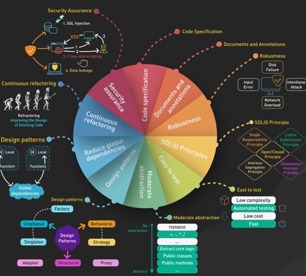
Comment - Code tells you how and comments tell you why.
Robustness - Code should handle unexpected situations without breaking. The exception to prevents crashing and unpredictable behavior. It should be defensive programming like thinking ahead and handle possible error.
Testing - Good code is not about how it work it is about how easy to test. Design components by thinking testing in mind.
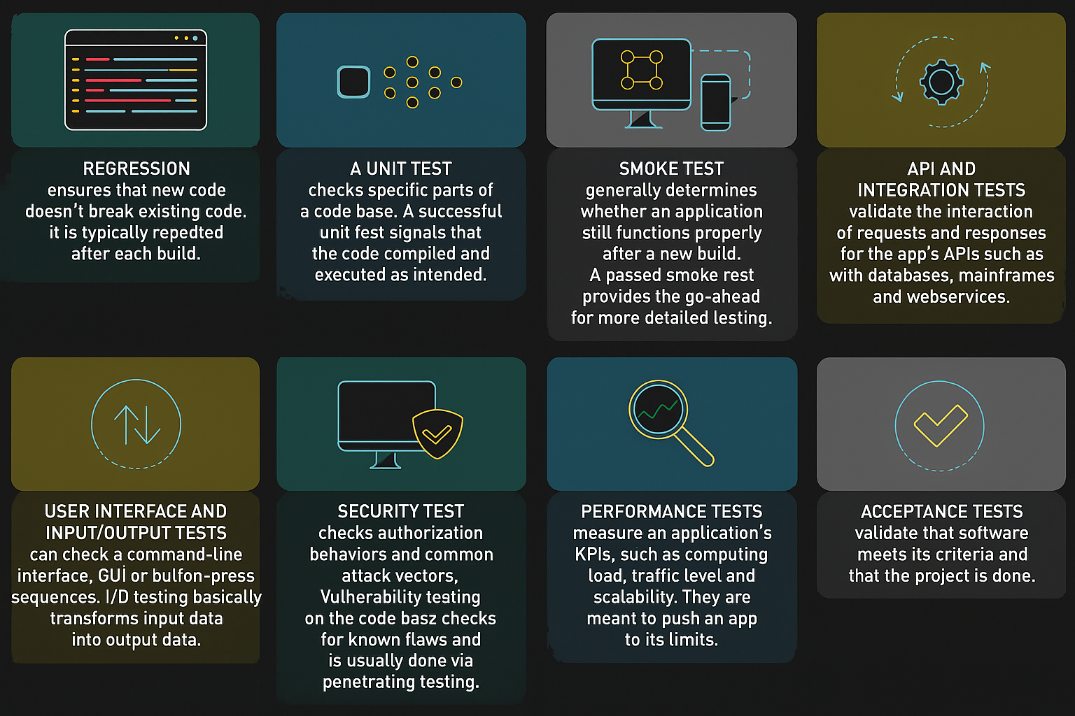
Refactor - It is the preventive maintenance for the code base. Solve the issue like duplicate code, improper naming.
Security - It should be taken care of the SQL injection and cross site scripting. To prevent it validate and sanitize user input. Use parameterized queries and output encoding.
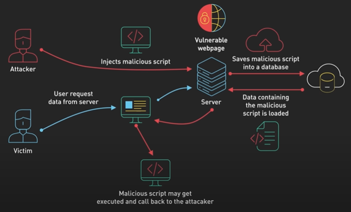
Popular API Protocol.
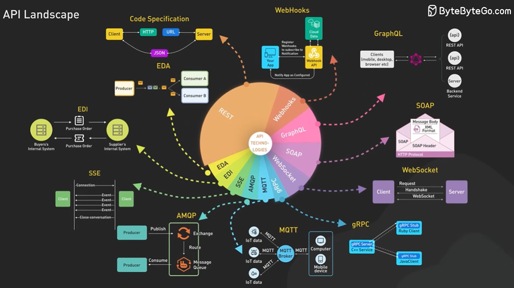
REST simple, scalable and works well with web services. It uses standard HTTP method and is a resource based approach and it is easy to use. It is stateless and scaling up is straight forward.
Rest has an issue with over fetching and under fetching data. When needed related data there will be multiple requests which will increase the latency. The graphQL works best.
GraphQL designed by Facebook is more flexible and efficient alternate to REST. All data will be retrieved with a single query and the frontend developers has more control on what data to fetch. It give control to the user by allowing them to make a single request and get the data they need. The data retrieval helps the problem of over fetching and under fetching.
It supports real time update to subscriptions keeping client updated in real time.
It is very dynamic and caching is difficult and hard to optimize the performance.
Webhooks are custom HTTP callbacks triggered by specific event within an applications. They do the real time communication between the system and removes the constant polling. It saves the computing power and bandwidth.
Webhooks supports decoupled architecture which supports modularity and scalability of the application.
SOAP has strict standard, strong security including authentication and authorization and encryption. XML based for the enterprise application.
Websocket is another protocol it establishes low latency bidirectional communication over a connection between client and server to facilitate its real time data transfer. It is idle for the applications where instant updates are critical.
gRPC build on the foundation of HTTP2. It uses protocol buffer to define service methods and message formats which allows services to expose custom methods much like functions in a programming language.
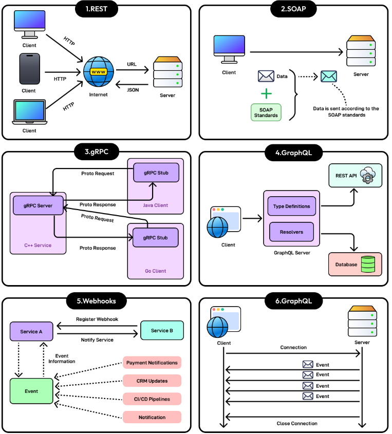
How Mobile apps are released.
https://youtu.be/RIX4ufelA58?si=-0oeGE_X5jr6XNAH
Releasing a mobile app can be tricky, with tough rules that could delay our launch. In this video, we’ll guide you through releasing an app on both iOS and Android. Grab a notepad—we’re about to share essential tips and tricks to navigate these challenges and release a smooth, efficient app that users will enjoy. Let’s get started! To start building our iOS app, we first need to join Apple’s Developer Program, which comes with an annual fee. For Android, we register as developers on the Google Play Console and pay a one-time registration fee. Next, we choose our programming language: Swift or Objective-C for iOS, and Java or Kotlin for Android. We write our apps with key development tools like Xcode for iOS and Android Studio for Android. Alternatively, we might opt for a cross-platform development tool like React Native or Flutter. These let us write code once and deploy it on both platforms. They can speed up development and reduce costs. However, they might not always offer the same performance or access to device-specific features as native development. Once we’ve written our code, it’s time to build and test. We compile our app’s binary and conduct thorough testing using tools like XCTest for iOS and Espresso for Android. Device farms help us to automate testing across hundreds of device configurations, catching issues that could affect different hardware or OS versions. This automation is integrated into our CI/CD pipelines to streamline the build and test process. Our goal is to deliver top-notch quality and performance across all devices, aiming for a rock-solid release candidate build ready for the next stage. It’s important to mention that while device farms like AWS Device Farm or BrowserStack provide significant benefits, they can be expensive. Their use might be planned later in the development cycle based on budget allowances and project requirements. Quality Assurance The next stage is QA. It starts with internal alpha testing to catch initial bugs, followed by “dogfooding,” where the team uses the app extensively. After this, we invite a group of users to try the app and provide feedback through beta testing platforms like Apple’s TestFlight and Google Play beta testing. It’s important to note that TestFlight limits us to 10,000 testers, and Google Play has similar constraints. We need to choose our external testers carefully to gain the most meaningful insights. These platforms help us gather feedback under real-world conditions and identify any issues that didn’t surface during earlier testing stages. Before we submit our app to the stores, we need to obtain internal approvals. This requires getting the green light from key stakeholders, focusing on criteria like UX consistency, brand alignment, and technical performance metrics. We also need to make sure our app meets all the necessary app store guidelines and adheres to industry regulations on security practices and privacy compliance. App Store Optimization is about making our app more visible in the app stores. It involves optimizing our app’s metadata, such as titles, descriptions, and keywords, and localizing our content for different regions to boost search rankings and attract more users. It’s also important to design eye-catching screenshots and icons that showcase our app’s best features. When it comes to release notes, get creative and highlight all the exciting new updates and improvements. Now comes the moment of truth: App Submission. For iOS, we submit our app through App Store Connect, closely following Apple’s strict guidelines. Android developers will proceed via the Google Play Console, adhering to Google’s policies. Prepare for potential delays and be patient—especially if this is a new app. The app review teams sometimes may seem unreasonably picky. They may request changes or additional information, so it’s important to allow extra time for this phase to ensure we secure approval. Finally, it’s time to release our app to the world! If possible, coordinate a simultaneous launch on both iOS and Android platforms. Make sure our marketing efforts are in full swing to generate buzz and anticipation for the launch. This can maximize our visibility and impact right out of the gate. But the journey doesn’t end there. Once our app is live, it’s crucial to monitor user feedback and analytics. We use this data to improve and update the app, fixing bugs and adding new features based on user demand. We also engage with users through reviews and social media to build a loyal community around the app. If you like our videos, you might like our system design newsletter as well. It covers topics and trends in large-scale system design. Trusted by 500,000 readers. Subscribe at blog.bytebytego.com.
KISS SOLID CAP BASE.
https://youtu.be/cTyZ_hbmbDw?si=6kAHZk7Cd70Syvjm
Ever wondered what CAP, BASE, SOLID, and KISS stand for? Let’s break down these system design acronyms and see how they help us build better software. The CAP theorem tells us that in any distributed data store, we can only guarantee two out of three of these properties: consistency, availability, and partition tolerance. Consistency means every read gets the most recent write or returns an error. Availability ensures that every request gets a response, even if it’s not the latest data. Partition tolerance means the system stays operational even when there are network faults. Imagine a distributed database where some servers can’t communicate with each other due to network issues, a situation known as “network partitioning.” If we prioritize consistency, some users might receive errors when accessing the database because not all servers have the latest data. But if we choose availability, every request will get a response, even if it might not reflect the most recent updates. The CAP theorem is often criticized for being too narrow, which brings us to the PACELC theorem. PACELC expands on CAP by considering latency as well. It states that if a partition happens (P), you must choose between availability (A) and consistency (C), like in CAP. But, “Else” (E), when there’s no partition, we still have to choose between latency (L) and consistency (C). If we use a globally distributed NoSQL database like Amazon DynamoDB, PACELC forces us to decide whether to prioritize low-latency responses over strong consistency. This brings us to a related concept - BASE. You’ve probably heard of the ACID principles for relational databases, where data needs to be Atomic, Consistent, Isolated, and Durable. However, with NoSQL databases, strict consistency isn’t always practical, especially in high-performance applications. That’s where BASE comes in. It stands for Basically Available, Soft State, and Eventual Consistency. “Basically Available” means the system appears available most of the time, even if some parts fail. Soft State implies that data might change over time due to the eventual consistency model. The system does not guarantee immediate consistency but reaches consistency over time. Eventual consistency means that the database doesn’t guarantee that all transactions are seen by all users immediately, but eventually, all reads will return the latest value. This allows for high scalability and replication, making it useful in scenarios where a slight delay in consistency is acceptable for faster response times and higher availability. Amazon DynamoDB is a good example of BASE principles in action. It prioritizes availability and latency for fast responses. Writes can be set to eventually consistent or strongly consistent, depending on how strict consistency is needed. While ACID principles are useful for scenarios requiring strong consistency, like financial transactions, BASE principles shine in large, distributed environments where availability and partition tolerance are prioritized. These principles provide more flexibility and resilience for large distributed systems. Let’s move on to SOLID principles, which help us write cleaner, more maintainable code. First up is the Single Responsibility Principle. It states that a class should only have one reason to change. This minimizes the impact of modifications. For example, separating user data management from user notifications ensures that changes in one don’t impact the other. Next is the Open/Closed Principle. Classes, modules, and functions should be open for extension but closed for modification. We can extend a module’s behavior without modifying its source code. It maintains code stability and reduces bugs. For instance, by using an interface for shapes, an area calculator can handle new shapes like circles and rectangles without modifying the core logic. Then there’s the Liskov Substitution Principle. It states that objects of a superclass should be replaceable with objects of subclasses without affecting the program’s correctness. This ensures that a subclass can stand in for its superclass without errors or unexpected behavior. For instance, separating flying behavior from a general Bird class ensures that non-flying birds like ostriches won’t cause errors. The Interface Segregation Principle states that clients should not be forced to depend upon interfaces they do not use. This encourages creating multiple, specific interfaces rather than a single, general-purpose interface. It prevents a class from being forced to implement interfaces it doesn’t use, reducing the side effects of changes in unrelated interfaces. For example, splitting a worker interface into specific ones like Workable and Eatable ensures that robot workers aren’t forced to implement unnecessary eating methods. Finally, the Dependency Inversion Principle states that high-level modules shouldn’t depend on low-level modules. Both should depend on abstractions. This principle aims to reduce the direct dependencies among different modules, making the system easier to modify and extend. For example, introducing a Database interface allows a program to work with various databases like MySQL and PostgreSQL without being tightly coupled to any specific implementation. And finally, KISS stands for Keep it simple, stupid. It’s a principle first used by the U.S. Navy in 1960. In software, it means systems work best when they’re simple, both in design and implementation. Google’s search interface is a good example of the KISS principle in action. The interface is famously simple, featuring only a logo, a search box, and a couple of buttons. This simplicity ensures that users are not overwhelmed and can focus on their primary task: searching. The straightforward design minimizes distractions and complications. So, next time we design a system, let’s remember that the best solutions might not come from adding complexity but from simplifying our design. If you like our videos, you might like our system design newsletter as well. It cover topics and trends in large scale system design. Trusted by 500,000 readers. Subscribe at blog.bytebytego.com.
Data Pipeline.
https://youtu.be/kGT4PcTEPP8?si=16Yj4LBm4dYdDYLp
Today, we’re diving into the world of data pipelines. So, what exactly is a data pipeline? In today’s data-driven world, companies collect massive amounts of data from various sources. This data is critical for making informed business decisions and driving innovation. However, raw data is often messy, unstructured, and stored in different formats across multiple systems. Data pipelines automate the process of collecting, transforming, and delivering data to make it usable and valuable. Data pipelines come in many different forms. The term is broad and covers any process of moving a large amount of data from one place to another. We present here a general version of it, but this is by no means the only way to implement an effective data pipeline. Broadly speaking, a data pipeline has these stages - collect, ingest, store, compute, and consume. The order of these stages can switch based on the type of data, but they generally have them. Let’s start at the top with data collection. Imagine we’re working for an e-commerce giant like Amazon. We get data flowing in from multiple sources: data stores, data streams, and applications. Data stores are databases like MySQL, Postgres, or DynamoDB, where transaction records are stored. For instance, every user registration, order, and payment transaction goes to these databases. Data streams capture live data feeds in real time. Think of tracking user clicks and searches as they happen using tools like Apache Kafka or Amazon Kinesis. Or data coming in from IoT devices. With all these diverse data sources, the next stage is the ingest phase, where data gets loaded into the data pipeline environment. Depending on the type of data, it could be loaded directly into the processing pipeline or into an intermediate event queue. Tools like Apache Kafka or Amazon Kinesis are commonly used for real-time data streaming. Data from databases is often ingested through batch processes or Change Data Capture (CDC) tools. After ingesting, the data may be processed immediately or stored first, depending on the specific use cases. Here, it makes sense to explain two broad categories of processing: batch processing and stream processing. Batch processing involves processing large volumes of data at scheduled intervals. Apache Spark, with its distributed computing capabilities, is key here. Other popular batch-processing tools include Apache Hadoop MapReduce and Apache Hive. For instance, Spark jobs can be configured to run nightly to aggregate daily sales data. Stream processing handles real-time data. Tools like Apache Flink, Google Cloud Dataflow, Apache Storm, or Apache Samza process data as it arrives. For example, Flink can be used to detect fraudulent transactions in real-time by analyzing transaction streams and applying complex event processing rules. Stream processing typically processes data directly from the data sources – data stores, data streams, and applications, rather than tapping into the data lake. ETL or ELT processes are also crucial to the compute phase. ETL tools like Apache Airflow and AWS Glue orchestrate data loading, ensuring transformations like data cleaning, normalization, and enrichment are applied before data is loaded into the storage layer. This is the stage where messy, unstructured, and inconsistently formatted data is transformed into a clean, structured format suitable for analysis. After processing, data flows into the storage phase. Here, you have several options: a data lake, a data warehouse, and a data lakehouse. Data lakes store raw, unprocessed data using tools like Amazon S3 or HDFS. Data is often stored in formats like Parquet or Avro, which are efficient for large-scale storage and querying. Structured data is stored in data warehouses like Snowflake, Amazon Redshift, or Google BigQuery. Finally, all this processed data is ready for consumption. Various end users leverage this data. Data science teams use it for predictive modeling. Tools like Jupyter Notebooks with libraries like TensorFlow or PyTorch are common. Data scientists might build models to predict customer churn based on historical interaction data stored in the data warehouse. Business intelligence tools like Tableau or Power BI provide interactive dashboards and reports. These tools connect directly to data warehouses or lakehouses, enabling business leaders to visualize KPIs and trends. Self-service analytics tools like Looker empower teams to run queries without deep technical knowledge. LookML, Looker’s modeling language, abstracts the complexity of SQL, allowing marketing teams to analyze campaign performance. Machine learning models use this data for continuous learning and improvement. For instance, bank fraud detection models are continuously trained with new transaction data to adapt to evolving fraud patterns. And that’s a wrap on the overview on data pipelines. If you like our videos, you might like our system design newsletter as well. It covers topics topics and trends in large-scale system design. Trusted by 500,000 readers. Subscribe at blog.bytebytego.com
Kafka vs RabbitMQ vs Messaging Middleware vs Pulsar.
Message Queue are software components enable different parts of the system to communicate asynchronously and they receiving messages they act in the middle allowing sender and receivers to work independently.
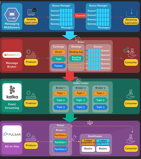
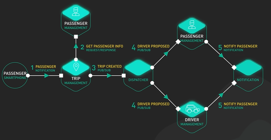
They are crutial for building scalable, loosely coupled and fault tolerance systems. They assure reliable communication handle async tasks in process high throughput data streams decoupling senders and receivers allow systems to scale independently and handle failures recently.
Example Uber - When a rider requests a ride the request enters the queue drivers are often matched to these requests this setup decomposed the riders request from the driver’s availability enabling efficient handling of numerous requests in real time.
Evolution of message queue architectures.
IBM MQ launched in 1993 pioneer enterprise messaging it provided reliable secure and transactional messaging for critical applications in finance and Healthcare large banks use ibm mq to process financial transactions reliably even during hardware failure.
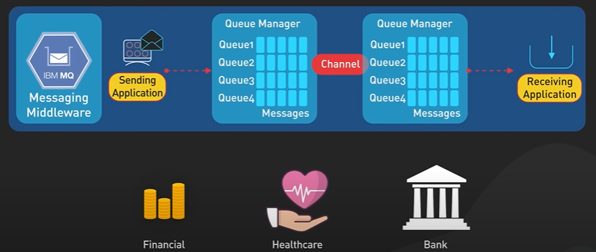
IBMF supports persistent and non persistent messaging it ensures. It offers robust transactions support to allow multiple messages to be grouped into a single unit of work which can be committed and rolled back as a whole.
It runs on a various platforms making it versatile for different enterprise environments.
Rabbit MQ releasing 2007 introduced a flexible and dynamic messaging model it supports multiple protocols including amp qp, mqtt and stomp.
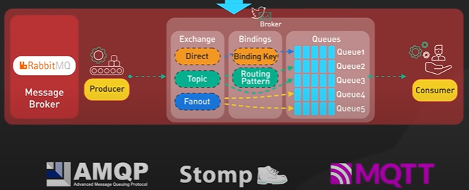
It offers features like message routing, queuing and pub/sub messaging.
Ecommerce platforms often use rapid mq for tasks like order processing and inventory updates improving system responsiveness and scalability.
RabbitMQ pluggins system allows user to extend functionality. It supports clustering for low distribution and high availability configurations.
Rabbit mq provides fine grain control over message acknowledgement ensuring reliable message processing.
Apache Kafka introduced in 2011 revolutionised message cues example high throughput real time data streaming Kafka offers a scalable and fault tolerant platform for handling massive data volumes. This unique architecture based on a distributed commit log enable event sourcing, stream processing in real time.
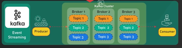
Kafka supports consumer groups for coordinated reading from the same topic by multiple consumers. It offers optional, exactly once semantics to prevent message loss or duplication.
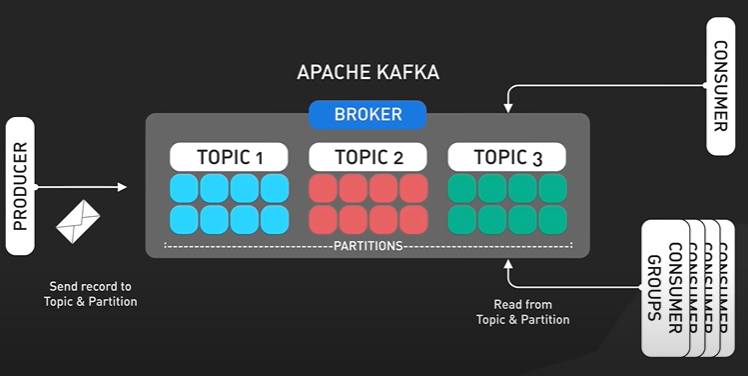
Apache Pulsar developer Yahoo combine character scalability and performance with the flexibility with rich features of traditional message queues. Its cloud native architecture, multi tenancy support and tiered storage works well in modern distributed computing environment.
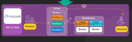
Pulsar is designed for multi tenancy allowing multiple tenants to share the same cluster while maintaining isolation and security.
It supports geo-replication, enabling data replication across multiple data centres for disaster recovery and data locality.
Pulsar’s tier storage allow older data to be offloaded to cheaper storage solitions like Amazon S3 reducing costs while maintaining access to historical data.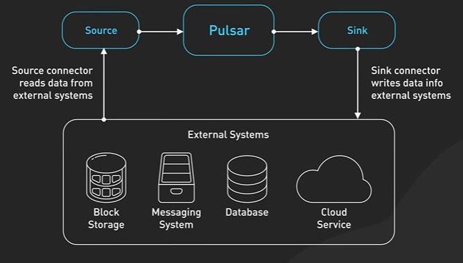
Strategies to scale the application.
7 must-know strategies to scale your database, one by one.
Indexing.
Indexes are like the index at the back of a book. They help you locate specific information quickly without having to scan every page. For example, in a customer database for an online retailer, indexing can quickly find customer orders based on order ID or customer ID. This allows customer service reps to pull up order histories quickly because these fields are indexed. The most common type of index is the B-tree index. B-tree indexes keep data sorted, making them ideal for a wide range of queries. They allow for fast insertion, deletion, and lookup operations. B-tree indexes are particularly effective for range queries, like finding all orders within a specific date range or retrieving customer records alphabetically by last name.
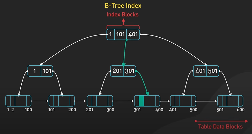
Indexes can significantly reduce query execution time. Without proper indexing, even a simple search query could turn into a full table scan, which is extremely time-consuming. However, it’s important to note that while indexes improve read performance, they can slow down write operations since the index needs to be updated whenever data is modified.
Finding the right balance and knowing which fields to index is key to maintaining optimal database performance.
Materialized views.
Think of them as pre-computed snapshots of data that are stored for faster access. They are especially useful for complex queries that would be too slow to compute on the fly every time. A real-world example is in business intelligence platforms like Tableau. Imagine a company needs to generate daily sales reports from a large dataset. Instead of querying the raw data every time a report is requested, which could take a long time, a materialized view can store the pre-computed sales data. This allows the reports to be generated quickly and efficiently. Materialized views can significantly improve performance by reducing the computational load on your database. However, they must be refreshed periodically to ensure the data remains up-to-date. This refresh operation can be resource-intensive, especially if the underlying data changes frequently. It’s important to balance the refresh frequency with the performance benefits they provide.
Denormalization.
Denormalization involves storing redundant data to reduce the complexity of database queries and speed up data retrieval. A common example of denormalization is social media platforms like Facebook. Facebook denormalizes data to store user posts and information in the same table. This approach minimizes the need for complex joins between tables, speeding up retrieval when displaying user feeds. While denormalization can significantly enhance read performance by simplifying query execution, it also comes with trade-offs. Storing redundant data means that updates must be carefully managed to maintain consistency across the database. This added complexity in maintaining consistent data can lead to potential issues if handled incorrectly.
Vertical scaling.
Vertical scaling involves adding more resources—such as CPU, RAM, or storage—to your existing database server to handle increased load. Consider a scenario where an online marketplace is experiencing rapid growth. Initially, their database server might handle the workload efficiently. However, as the user base and transaction volume increase, the server starts to struggle with the load. To address this, they upgrade their database server by adding more powerful CPUs, increasing the RAM, and expanding the storage capacity.
Additionally, vertical scaling doesn’t address redundancy; a single server failure can still bring down your database.
Caching.
Caching involves storing frequently accessed data in a faster storage layer to reduce the load on your database and speed up response times. For example, consider an online streaming service like Netflix. When users browse through movie titles, Netflix retrieves movie metadata from a cache rather than querying the database each time. This approach drastically reduces the time it takes to display movie information, providing a more seamless user experience.
Caching can be implemented at various levels, such as in-memory caches using tools like Redis or Memcached, or even at the application level with built-in caching mechanisms. However, caching also has its challenges. One major consideration is cache invalidation—ensuring that the cache remains up-to-date with the most recent data. If the cached data becomes stale, users might see outdated information. Therefore, it’s essential to implement strategies for refreshing the cache appropriately, either through time-based expiration or event-driven updates.
Replication.
Replication involves creating copies of your primary database on different servers to improve availability, distribute the load, and enhance fault tolerance. Replication can be configured in several ways, such as synchronous or asynchronous replication.
In synchronous replication, data is copied to the replica servers simultaneously as it’s written to the primary server, ensuring immediate consistency. However, this can introduce latency as the primary server waits for all replicas to confirm the write operation.
In asynchronous replication, the primary server doesn’t wait for replicas to confirm the write, which improves performance but may lead to temporary inconsistencies.
While replication enhances read performance and availability, it introduces complexity in maintaining data consistency, especially in distributed systems. Additionally, replication increases the storage and maintenance overhead, as multiple copies of the database need to be managed and synchronized.
Sharding.
Sharding is a database architecture pattern that involves splitting a large database into smaller, more manageable pieces, called shards. Each shard is a separate database that contains a subset of the data. For instance, consider a popular social media platform like Instagram. With millions of users generating content every second, a single database can’t handle the load efficiently. To address this, Instagram shards its database by user ID, meaning each user’s data is stored on a specific shard. This way, the workload is distributed across multiple servers, improving performance and reliability. Sharding is particularly effective for scaling databases horizontally. Instead of upgrading a single server’s hardware, you can add more servers to distribute the load. Each server handles a portion of the data, which significantly enhances both read and write performance. However, sharding introduces complexity in database design and management. Deciding on the right sharding key is crucial to ensure an even distribution of data and workload across shards. Querying across multiple shards can also be complex and may require changes to your application’s query logic. Additionally, re-sharding—redistributing data when shards become imbalanced—can be a challenging and resource-intensive process. Despite these challenges, sharding remains one of the most effective ways to scale large databases. It allows for efficient handling of massive amounts of data and high query loads by spreading the data across multiple servers.
Concurrency vs Parallelism.
How grab the headers multiple tasks by processing user input reading the difference between these concepts is essential for building efficient and responsive applications .
That’s our concurrency imagine a programme that handles multiple tasks by processing user inputs reading files and making network requests concurrency allows your programme to juggle this task efficiently even on a single cpu core here’s how it works the cpu ratios switches between tasks working on each one for a short man of time before moving to the next this process known as context switching creation illusion that tasks are progressing simultaneously though they are not think of it like chef working on multiple dishes they prepare dish for dirt this went to another and keep alternating while the dishes are finished simultaneously progress is made on all of them however contact switching comes with overhead the cpu must say that we store the state of each task which takes time excessive contact switching can hurt performance now let’s talk about parallelism this is where multiple tasks executed simultaneously using multiple cpu cores each core handles a different task independently at the same time imagine the kitchen with two chefs 1 chopped vegetables while the other could meet both chaps happen in parallel and the meal is very faster the system design concurrency is great for tasks that involve waiting like IO operations it allows other tasks to progress during the wait improving overall efficiency for example the Web Server can handle multiple requests concurrently even on a single core in contrast parallelism excels at heavy computations like data analysis or rendering graphics these tasks can be divided into smaller independent subtasks and execute simultaneously on different cores significantly speeding up the process let’s look at some practical examples web applications use concurrency to handle user inputs database queries and background tasks movefully providing a responsive user experience machine learning leverages parallelism for training large models by distributing the training data across multiple cores or machines you can significantly reduce competition time video rendering benefits from parallelism by processing multiple frames simultaneously across different cores speeding up the rendering process scientific simulations utilise parallelism to model complex phenomena by whether patterns or molecular interactions across multiple processors big data processing frameworks such as Hadoop and spark leverage parallelism to process large studies as quickly and efficiently this is important to note that while concurrency and parallelism are different concepts they are closely related concurrency is about managing multiple tasks at once a lot of parallelism is about executing multiple tasks at once concurrency can enable parallelism by structuring programmes to allow for efficient parallel execution using concurrency we can breakdown a programme into smaller independent tasks make it easier to take advantage of parallelism these concurrent tasks can be distributed across multiple cpu cores and executive simultaneously so while concurrency doesn’t automatically lead to parallelism it provides a foundation that make parallelism easier to achieve programming languages with strong concurrency primitives simplify writing concurrent programmes that can be efficiently parallelized concurrency is about efficiently managing multiple tasks to keep your programme responsive especially with IO bank operations parallelism focuses on boosting performance by handling computation heavy tests simultaneously by understanding the differences in interplay between concurrency and terrorism and leveraging the power of concurrency to enable parallelism we can design more efficient systems and create better performing applications.
Linux Crash Course - Understand file permission.
Permission to maintain the file control in linux environment.
Ownership - Every file has 3 types of owner - Owner(users), Group and Others.
User - the owner who created the directory. They have the most control over it.
Group - consists of users who share the same permission to access the file or the directory.
Others - who are neither the owner or the members of the group.
To manage access linux uses 3 types of permissions - Read(r), Write(w) and Execute(x).
Read - allows users to open and read file content.
Write - allows modifying and editing file content.
Execute - allows the file to run as a program.
Permissions are represented in three ways binary, octal and string representation.
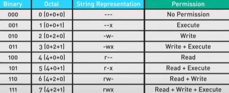
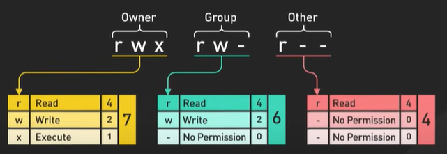
Considering the permission rwx - 111 in binary. In octal 7(read 4, write 2 and execute 1).
Using the chmod 764 sample.txt command we can set the permission of the file.
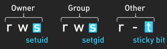
Special Permission Bit.
The Special permission bit provides additional control over the files and directories.
The setuid bit when set on an executable files allows it to run with the permission of the file owner, not the user running the file. This is useful for tasks that require higher privileges.
For example the password command which changes the user password has the setuid bit set. This allows regular users to change their password.
ls -l /usr/bin/passwd
-rwsr -xr -x. 1 root root 27832 June 10, 2006 /usr/bin/passwd
When they setuid bit is set the execute bit for the owner shows as s in -rwsr. The bit can be set on files and directories.
The setgid bit can be set on files or directories. On an executable file, it allows the file to run with the permission of the group that owns the file. On a directory, it ensures that new files and subdirectories created within the directory inherit the group ownership of the directory.
This is useful for shared project directory ensuring all files created within have the same group ownership, allowing team members the necessary access permissions. When they setgid bit is set the execute bit for the owner shows as s in -sr.
ls -l /usr/bin/write
-rwxr -sr -x 1 root tty 19536 August 4, 2006 /usr/bon/write.
The sticky bit when set on a directory ensures that only the file owner the directory owner Or the root user can delete or rename the file within the directory.
It is commonly used on directory like /tmp to prevent users from deleting each others file.
dr wx rwx rwt
When the sticky bit is set the execute bid for others is shown as t.
To set the special permission we can use the CHMOD command with specific symbol or numeric representation.
For setuid use u+s or 4
For setgid use g+s or 2
For sticky bit use +t or 1
Example we want to set the setuid bit on an executable file named important_script

In the command 4 set the setuid bit, 7 gives the owner read, write and execute, 5 gives group and others read and execute permissions.
Session vs JWT.
First let’s walk through the flow of session based authentication the user says they’re logging credentials to the server the server verifies these credentials if they’re valid it creates a new session the server then stores the session data typically in a database or in memory cache like Redis this data may include user id session exploration time and other metadata the server sense packet response with a unique session id usually in the form of a cookie on subsequent requests the clients automatically sends the session id token with each request the server takes the session id looks at the corresponding session data in the session store and uses that data to authenticate and process the request the key point is that recession based authentication the server is responsible for creating and storing the session data it uses the session id as a key to retrieve this data on future requests 1 advantage of sessions is that revoking a session is straightforward since the session data is stored on the server the server can simply delete or invalidate the session at anytime however in a distributed system where your application runs on multiple servers all those servers need access to the same session data this is typically achieved by using a centralised session store that all servers access like Redis or distributor sql database all this works well it does add some complexity and potential in C to each request as the server needs to make a separate trip to the session store now let’s look at the flow of job base of the location first the issue says they are locking credentials to the server the server verifies these credentials if they are valid it generates a job the server sides the jot with a secret key this signature ensures the integrity of the token preventing tempering the server that sends back the job to the client typically in the response body the client source to jot usually in local storage or in cookie on subsequent requests the client says to jog in the request headers the server verifies the jot signature it is valid the server trusted data in the token and uses it for authentication authorization the critical difference here is that with jobs the server doesn’t store any session state or the necessary data is contained within the token itself.
Which is store on the client this makes charts stainless for signing charts there are several algorithms available with Hmac Rsa and ect being the most common symmetric signing method which means that the same secret key is used to sign and verify the token this is simpler and more efficient but it requires sharing the secret key with any service that needs to verify the token which can be a security concern rsa and ectsa on the other hand are asymmetric signing methods they use a private key to sign a token in a public key to verify it this allows for a more secure architecture where the private keys kept secret and only used for signing while any service can verify the token using the public key however this **** complexity and computational overhead compared to Hmac the choice of signing algorithms depends on your security requirements and system architecture if you have a monolithic application or trust all the services in your system each mac might be sufficient but if you have a microservices architecture or need to share jobs with untrusted 3rd party services rsa or ecdsa provide a more secure solution 1 talent with jobs is handling token exploration if a token is stolen it can be used until it expires to mitigate this you can use refresh tokens in combination with short lived access tokens the access token is the actual job useful authentication on issue request it has a short expiration time typically around 15 minutes the refresh token on the other hand has a much longer expiration time perhaps several days or weeks when access token expires instead of requiring the use of the login again the client can send a refresh token to a special token endpoint on the server the server cheques if the refresh token is valid and hasn’t been revoked if everything cheques out the server issues a new access token this process happens behind the scenes without requiring indirection from the user this approach strikes a balance between security and user experience the short lived access token limit the window of potential misuse if a token is stolen while the long lived refresh token allow users to remain authenticated for an extended. Without needing to lock in repeatedly it’s important to note that the refresh token is only sent when the access token has expired not on every request the access token is sent on every request that we require authentication so why should you use session based authentication and when adjust a better choice session based authentication is a good fit when you need the ability to revoke sessions instantly if a user reports that can is compromised you can immediately invalidate a session on the server side sessions are a good choice if you already have a centralised data store for other purposes in this case you can leverage that existing infrastructure for session storage as well however it’s important to keep in mind that using a centralised session store does **** latency to each request as the server needs to fetch the session data from the store finally sessions keep sensitive data on the server which can be a security advantage on the other hand just a great choice when you need a stylus architecture because just store all the necessary data in the token itself your server doesn’t need to keep track of sessions in memory or in the database this makes it much easier to scale your application horizontally across multiple servers charts are also useful when you need to share authentication data with other services for instance in a microservices architecture a chat generated by a authentication service can be verified and trusted by other services without needing to contact the authentication service on each request if you do choose dots consider implementing refresh tokens to balance security and user experience refresh token allows you to use short lived access token to limit the window of potential misuse while still allowing users to remain authenticated for the extended. Ultimately the choice depends on the specific needs and architecture of your applications.
Papers to understand.
In this video, we’ll explore 25 research papers that have made a huge impact on computer science. We’ll put these groundbreaking papers into groups to make them easier to understand. For each paper, we’ll talk about the key ideas and why they matter, giving you a quick overview of their significance. So, let’s get started! First up, let’s check out the papers that changed the game for distributed systems and databases. The Google File System paper introduced a highly scalable distributed file system built to handle massive data-intensive applications. GFS can handle failures while using inexpensive commodity hardware, and it delivers high performance to many users. It’s different from traditional file systems because it expects failures to happen, optimizes for large files that are frequently appended to and read sequentially, and uses chunk replication to keep data safe. This innovative approach has set the stage for modern big data processing systems. The Amazon Dynamo paper introduced a highly available key-value store designed to scale across multiple data centers. By prioritizing availability over consistency in certain failure scenarios, Dynamo uses techniques like object versioning and application-assisted conflict resolution to maintain data reliability. This approach has inspired many other NoSQL databases, including Amazon’s own DynamoDB. BigTable and Cassandra demonstrated what distributed NoSQL databases could do by efficiently managing structured data at a massive scale while ensuring high availability and fault tolerance. BigTable, developed by Google, is known for its low-latency performance and scalability, making it perfect for large-scale data processing and real-time analytics. On the other hand, Apache Cassandra, initially designed at Facebook, combines features from Amazon’s Dynamo and Google’s BigTable, offering a highly scalable, multi-master replication system with fast reads and writes. Google’s Spanner improved distributed databases by offering a globally consistent, highly available, and scalable system. It introduced the TrueTime API, which uses time synchronization to enable consistent snapshots and multi-version concurrency control, supporting powerful features like non-blocking reads and lock-free read-only transactions. FoundationDB introduced a new way to handle distributed transactions with its multi-model, key-value store architecture. It is known for its ACID transactions across a distributed system, providing strong consistency and support for various data models. FoundationDB’s layered design supports multiple data models on top of a single, robust core, making it very adaptable. Amazon Aurora pushed the limits of high-performance databases by separating storage and compute. This design allows for scalable and resilient storage that can automatically grow and shrink as needed. Aurora also provides high availability and durability with six-way replication across three availability zones, ensuring data integrity and fault tolerance. Next, let’s talk about the papers that changed data processing and analysis. Google’s MapReduce revolutionized big data processing by enabling the parallel processing of huge datasets across large clusters of commodity hardware, making it easier to handle parallelization, fault tolerance, and data distribution. Apache Hadoop, an open-source version of MapReduce, became a popular choice for big data processing tasks, using the same principles to handle large-scale data efficiently Flink brought together stream and batch processing, allowing for the seamless processing of real-time and historical data. It provided a powerful framework for building data-intensive applications by treating batch processing as a special case of streaming, offering consistent semantics across both types of data processing. Apache Kafka, developed by LinkedIn, has become the leading platform for distributed messaging and real-time data streaming. It enables the creation of reliable, scalable, and fault-tolerant data pipelines. It organizes data into topics, with producers publishing data and consumers retrieving it, all managed by brokers that ensure data replication and fault tolerance. Kafka’s high throughput and low latency make it ideal for applications requiring real-time data processing. Google’s Dapper paper introduces a distributed tracing system that helps troubleshoot and optimize complex systems by providing low-overhead, application-level transparency. It highlights the use of sampling and minimal instrumentation to maintain performance while offering valuable insights into complex system behavior. Google’s Monarch is an in-memory time series database designed to efficiently store and query huge amounts of time series data. It features a regionalized architecture for scalability and reliability, making it ideal for monitoring large-scale applications and systems by ingesting terabytes of data per second and serving millions of queries. Moving on, let’s explore the papers that tackled complex challenges in distributed systems. Google’s Borg paper explained how Google manages its large-scale clusters. It introduced the concept of containers and showcased the benefits of a centralized cluster management system. Uber’s Shard Manager provides a generic framework for managing sharding in distributed systems. It simplifies the process of scaling and managing large-scale databases by adaptively adjusting shard placement in response to failures and optimizing resource utilization. Google’s Zanzibar is a global access control system. It efficiently manages access control lists across large-scale distributed systems. It provides a uniform data model and configuration language to express diverse access control policies for various Google services. Zanzibar scales to handle trillions of access control lists and millions of authorization requests per second. Facebook’s Thrift paper explores the design choices behind their code-generation tool. It highlights the benefits of using a common interface definition language to build scalable and maintainable systems. The Raft Consensus Algorithm provided an easier-to-understand alternative to Paxos. It simplified the process of building fault-tolerant distributed systems. The important 1978 paper, “Time, Clocks, and the Ordering of Events in a Distributed System,” introduced the concept of logical clocks. It establishes a partial ordering of events in distributed systems, providing a framework for synchronizing events and solving synchronization problems without relying on physical clocks. Now, let’s explore papers that introduced groundbreaking concepts and architectures. “Attention Is All You Need” introduced the transformer architecture in 2017. It has had a huge impact on natural language processing. The paper show how effectiveness self-attention mechanisms are. They allow models to weigh the importance of different words in a sentence. This innovation led to powerful language models like GPT. They have significantly improved tasks such as translation, summarization, and question-answering. The Bitcoin whitepaper laid the groundwork for cryptocurrency and blockchain. It introduced the concept of a decentralized, peer-to-peer electronic cash system and sparked a new era of digital currencies and decentralized applications. “Go To Statement Considered Harmful,” published in 1968, challenged conventional wisdom and sparked important discussions about programming language design. It argued against the use of the “go to” statement and advocated for structured programming practices. Finally, let’s discuss some papers that focused on specific applications and optimizations. The Memcached paper showcased the complexities of caching at scale. It highlighted the challenges and solutions in building a distributed caching system to improve application performance. The MyRocks paper presented an LSM-tree-based database storage engine. It demonstrated how to optimize storage and retrieval operations for large-scale databases. Twitter’s “Who to Follow” service gave insights into building effective recommendation systems. It showcased the algorithms and techniques used to generate personalized user recommendations based on social graph analysis. The 2021 survey on vector databases offered an insightful look into this cutting-edge technology. It covered the basics, how they are built, and their various uses. It focused on how these databases are designed to handle and search complex, high-dimensional data efficiently. These papers represent just a fraction of the amazing research that has shaped computer science. They help us gain a deeper appreciation of the challenges, solutions, and innovations that have brought us to where we are today. If you like our videos you might like a system design newsletter as well. It covers topics and trends in large scale system design. Trusted by 500,000 readers. Subscribe that blog.bytebytego.com.
Linux Performance Tools.
https://youtu.be/iJ_eIsA5E1U?si=lV7qTx3rNLMjdpyC
today we explore essential tools and techniques to help us efficiently diagnose and solve performance issues on leux systems before we dive into the technical details let’s talk about a crucial First Step that even season developers sometimes Overlook verifying that there’s actually a real performance problem when someone reports a performance issue we need to ask probing questions what make us think there’s a problem has the system ever performed better what recent changes might have affected performance can we quantify what slow means in this context is the issue affecting multiple users or just one these questions aren’t just formalities they help clarify the issue establish a baseline for comparison and sometimes even resolve the problem without further investigation let me share a quick real world example a developer once complained about a slow database query taking 5 seconds after investigating we found this query had always taken 5 Seconds the issue wasn’t performance but mismatch EXP expectations imagine if I jump right into troubleshooting without asking questions I would have wasted time and resources chasing a non-existent problem in other repair they call this the ports Cannon approach blindly replacing ports hoping to fix an issue this highlights why is critical to confirm there’s a genuine performance problem before diving into analysis it saves time and keeps us focused on solving actual issues not Chasing Ghosts once we confirm a genuine performance issue we need to Define it precisely this means moving beyond vague terms like slow to specific metrics are web pages taking 10 seconds to low are database queries timing out we need to pinpoint when and where these issues occur we also need to understand the scope and impact is this affecting all servers or just one how many users are impacted and what’s the business consequence finally we investigate a source of the problem is a low coming from legitimate user activity a specific application or perhaps a runaway process we quantify this in terms of requests per second data transfer rates and how this change over time this focused approach creates a clear road map for our investigation ensuring we don’t waste time on unrelated areas now let’s look at some basic tools that can help us gather this information and pinpoint the root cause of our performance issues we’ll start with uptime the key metric here is the low average which shows the average number of processes that are either running or waiting for resources over the last one five and 15 minutes is a complex metric that can be influenced by various factors if these numbers are consistently higher than the number of CPU cores it might indicate that processes are competing for resources but it’s not always straightforward high low averages can be caused by CPU intensive tasks IO bottlenecks or even short livv process that quickly come and go remember that the low average alone doesn’t tell tell the whole story it’s more a starting point that tells us we might need to investigate further when we see elevated low averages this are C to dig deeper with other tools this brings us to the next Tool top top provides a dynamic continuously updated view of the systems processes and key metrics it’s like a dashboard for A System’s performance some key indicators to watch are the percentage of CPU usage by user processes and system processes top also shows a list of running processes pay close attention to any processes consuming an unusually high percentage of CPU or memory this could be the culprit behind performance issues remember top give us a snapshot of the current moment for a fuller picture we might need to watch it over time or use other tools to complement your analysis next up is VM stat VM stat shows multiple system components at once updating in real time key areas to watch includes the CPU Q ioe swap activity and IO wait time in the CPU section for a deeper di into this iio return to iio stat it give us a continuous view of this activity key metrics to watch are transactions per second for this activity and the percentage of time spend waiting for Io operations in the CPU section iio step breaks down IO operations by device this is useful when we need to identify which specific disc is causing performance issues now let’s Explore Net a useful tool for monitoring network connections net stat has many options we’ll focus on a few useful ones for performance analysis first let’s list all active connections this command displays all active connections both incoming and outgoing it’s helpful for identifying open ports and active services on our system we can display only listening ports we can also count connections for a specific Port here we’re counting connections on Port 80 this quick can can help us gauge the low on a particular service it we see a unusually high number of connections it might indicate a potential performance issue a traffic Spike that needs investigation last but not least let’s look at SAR which stands for system activity reporter it’s a versatile tool that’s great for historical data here’s an example of how it reports CPU usage while s provides similar information to other tools we’ve discussed what sets it apart is his ability to save historical d data many Linux distributions configure s to collect data periodically this automated data collection can be invaluable if users report intermittent slowdowns we can use S to look back at previous dayses and spot performance Trends it’s particularly useful for correlating system performance with specific times or events it might identify patterns not obvious in real-time monitoring it’s important to stress that we are just scratching the service here the Linux performance landscape is is vast there are tools for every level of the system from Hardware all the way up to applications and for every subsystem from file systems to network Stacks remember this process is iterative we might need to use multiple tools and dig deeper depending on what we find the key is to start broad with tools like up time and top then narrow our Focus based on what we discovered if you enjoy our videos you will love a system design newsletter we cover important topics in trans in large scale system design join our community of 1 million subscribers from the tech industry subscribe at blog. bio.com
How Internet works.
The internet started with ARPANET in 1960s. The TCP IP is founded in 1970s. The Email and DNS started in 1980s and WWW in 1990s. In 2000s the mobile internet Tand social media.
The key components of the internet.
The network Edge - The network Edge consists of end systems also called hosts these are the devices connected to the internet they include desktop computers servers mobile devices and an increasing number of iot devices like smart home appliances, hosts are some sometimes divided into two categories client and servers.
Clients are typically personal devices like PC and smartphones servers are usually more powerful machines that store and distribute web pages stream video relay email and provide similar services.
Today most of the servers providing search results email web pages and videos reside in large data centers these data centers can house thousands of interconnected servers forming the backbone of many internet services.
Access networks these physically connect end systems to the first router on a path to other distance and systems.
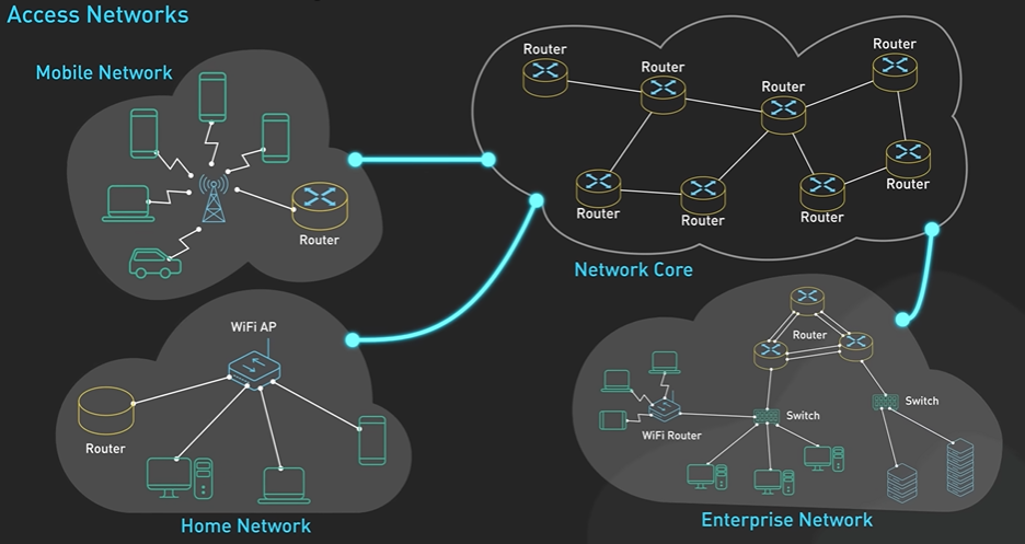
There are three main types of access networks - home access networks these enable connectivities within a residential environment they typically use technology like DSL cable internet or Fiber Optic connections to link homes to the broader internet.
Institutional access networks used by organizations and businesses these are designed to handle the specific needs and requirements of large scale operations they often use high-speed fiber optic connections and complex Network architectures to support many users and data intensive applications.
Mobile access networks which enable our smartphones to connect to the internet these are cellular Technologies like 5G to provide wireless internet access.
The network core this is the mesh of packet routers and links that interconnect the internets and systems at the heart of the network course a routers specialized devices that direct packets from one network to another.
These routers handle the task of packet forwarding which ensures data reaches its intended destination efficiently.
The network course operates based on the principle of packet switching - when send an email or lower web page the data doesn’t travel as a single continuous stream instead it’s broken down into smaller chunks called packets. Each packet contains a portion of the data along the information about its source and destination these packets are then sent independently through the network they may take different routes and arrive at different times.
Once all the packets reach the destination they reassemble into the original message this method has several advantages it allows the network to handle multiple Communications simultaneously making efficient use of the available bandwidth it also provide resilience if one route is congested or fails packets can be rerouted through different paths.
There are two key functions performed inside the network core forwarding and routing.
Forwarding is the local action of moving an arriving packet from a router’s input link to the appropriate router output link it’s controlled by a forwarding table inside each router.
When a packet arrives the router examines the packet destination address and uses his forwarding table to determine which output links to send the packet to.
Routing on the other hand is the global process of determining the full paths packets take from source to destination.
Internet routing algorithms compute the shortest and most efficient paths between any two points on the global Network. These algorithms take into accounts factors that network topology, traffic conditions and link capacity to make routing decisions.
One of the most important routing protocols on the Internet is BGP Border Gateway Protocol. BGP is used to exchange writing informations between different autonomous systems large networks or groups of networks typically managed by isps or large organizations in essence bgp allows each as to announce which IP address ranges it can reach and this information propagates across the internet .
The routing process is dynamic and adaptive if a link fails or become congested routing algorithms can quickly recalculate paths to ensure data continues to flow efficiently across the network.
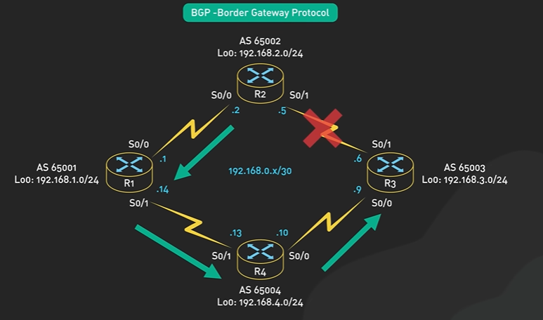
All activity on the internet involving Communications between network devices is governed by protocols.
Protocols are standard rules that Define message formats ordering of message exchanges and expected responses they are like the language and grammar of the internet to ensure that different devices and systems can understand each other some common protocols include TCP UDP IP and HTTP.
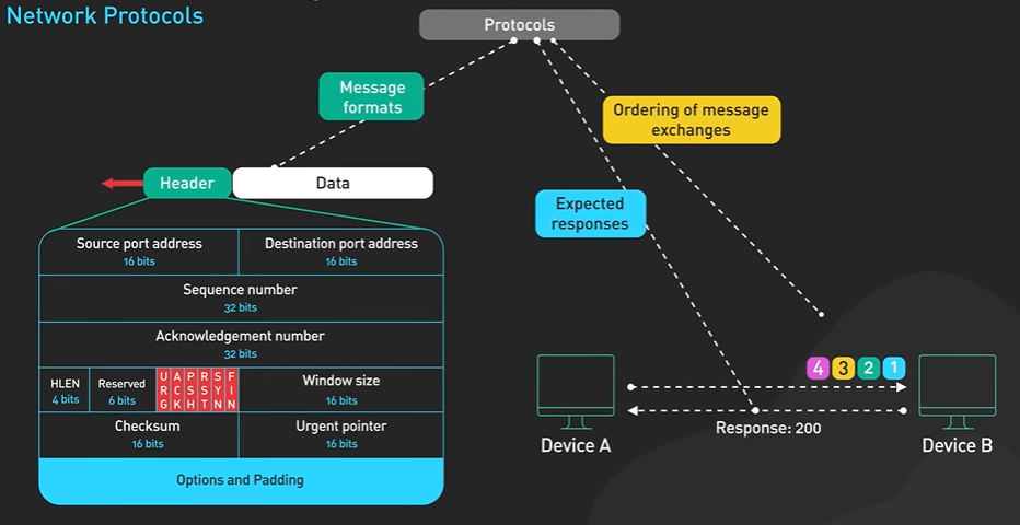
TCP ensures reliable order delivery of data between applications it handles things like breaking data into packets, acknowledging received packets and retransmitting lost packets.
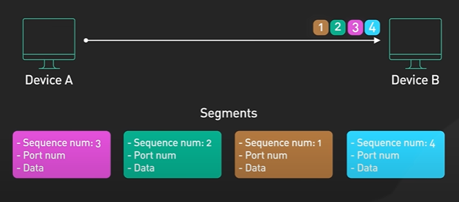
IP on the other hand is responsible for addressing and routing packets across the internet. Every device connected to the internet has an IP address which acts like a postal address for data packets.
HTTP is the protocol that powers the worldwide web defining how messages are formatted and transmitted between web browsers and servers.
A URL into your browser essentially sending an HTTP request to a web server these protocols and many others work together to enable the complex interactions that occur every time you send an email stream a video or browse a website.
Internet Protocol stack also known as a tcpip stack is a conceptual framework that standardize the protocols used for communication over the Internet. The tcpip stack typically consists of four layers - Application layer, Transport Layer, Network Layer and Link Layer.
The top we have the application layer closest to the end user and interacts directly with software applications protocols in this layer include HTTP for web browsing SMTP for email and FTP for file transfers.
The transport layer it ensures reliable data transfers between applications the two main protocols in this layer are TCP and UDP TCP provides reliable order delivery of data while UDP offers faster but less reliable transmission.
The IP layer this handle the addressing and routing of data packets across different networks the main protocols here are IPV4 and IPV6 which Define how data should be packetized, addressed, transmitted routed and received.
The link layer it manages the physical connection between devices on the same network segment. This layer deals with the hardware aspects of network communication including network interface cards and device drivers.
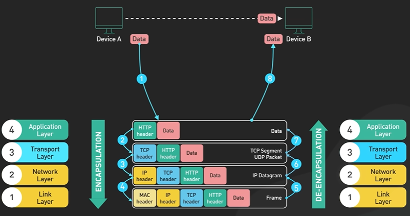
Send data it starts at the application layer and moves down through each layer each layer adds its own information to the data a process called encapsulation when the data reaches its destination it moves up through the layers with each layer stripping off its information a process called decapsulation.
HTTP1 HTTP2 HTTP3.
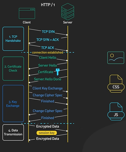
There is a TCP handshake security and all happens for every resource, image, file.
today we’re diving into the fascinating world of HTTP it’s the backbone of the web we explore how it evolved from HTTP 1 to two and then to three get ready for an interesting ride HTTP stands for hypertext transfer protocol is how browsers talk to web servers they ask for web pages and get them back at first HTTP was for hypertext documents these are documents with links to other documents but developers soon found HTTP could send imag and videos too now it’s also used for apis file transfers and a wide range of webbased services let’s go back to 1996 that’s when HTTP 1 was introduced but before that there was HTTP 0.9 it was simple it only supported get and had no headers it only sent HTML files there were no HTTP headers or status codes HTTP 1.0 edit headers status codes and new methods that post and head it was straightforward the browser would ask for a web page the server would send it each request needed its own connection this means a lot of back and forth it wasn’t very efficient he’s why first there’s a TCP handshake is a three-way process to start a connection then for https there’s a TLS handshake for security this all happens before any data is sent with HTTP 1 this happened for every resource every image CSS file file or JavaScript file not ideal right in 1997 HTTP 1.1 came out it fixed problems with http1 it’s still used a lot today even after 25 years why it has some great new features HTTP 1.1 introduced persistent connections the connections stay open unless to to close this meant no more closing after every request no more multiple TCP handshakes it got rid of the extra work of constantly opening and closing connections it also introduced pipelining this L clients send multiple requests over one TCP connection they didn’t have to wait for responses for example when a browser needs two images he can request them one after the other this made things faster it reduced the wait time for each response another key feature was chunk transfer encoding servers could send responses in smaller chunks they didn’t have to wait for the whole response to be ready this may initial page rendering faster it improved user experience especially for large or dynamic content HTTP 1.1 also brought better caching and conditional requests it added headers like cash control and eag these help manage cash content and reduce unnecessary data transfers conditional request using headers like if modify sins let clients request resources only if they changed this save bandwidth and improved performance but websites grew bigger and more complex the this showed a big problem with HTTP 1.1 had outline blocking if the first request in the pipeline was delayed all the others had to we because of this and other issues many browsers didn’t use pipelining developers found ways around these limits one was domain Shing websites would serve static asset from subdomains each new subdomain got six more connections another trick was to make Fel request by bundling assess images would be combined using Sprites CSS and JavaScript files would be concatenated in 2015 http2 arrived it was designed to fix HTTP 1’s performance problems it brought major improvements HTTP 2 introduced a binary framing layer unlike HTTP 1’s plain text messages http2 uses binary format messages are divided into smaller units called frames these are send over the TCP connection the binary framing layer handles all this http2 also brought full request and response multiplexing clients and servers can break down HTTP messages into independent frames these can be mixed during transmission and put back together on the other side this fixed the head align blocking problem from http1 stream prioritization was another key http2 feature the order of loading assets matters for web pages stream prioritization lets developers set the importance of requests the browser can tell the server which asset of high priority the server then sends more frames for these important requests http2 also supports server push http2 allows multiple responses to client’s request a server can send extra resources along with the requested HTML page is like giving the client a resource before they even ask for it lastly htb2 introduce header compression in http1 only the main data was compressed headers were sent as plain text http pp2 uses xack to make headers smaller xack compresses headers and remembers past headers it uses this info to compress future headers even more but as web apps got more complex and mobile internet became common httv 2 shows some limits tcp’s nature is handling of packet lws and head outline blocking caused lower page lows this was especially true on high latency or lossy networks this led to http 3 standardizing in 2022 HTTP 3 used quick instead of TCP quick was developed by Google it was built on UDP a connectionless protocol UDP doesn’t need to set up a connection before sending data quick and HTTP 3 have some big advantages they reduce latency they improve multiplexing without TCP head outline blocking they handle packet loss better they perform better on mobile networks with seamless connection changes when a client connects to a server with http p 3 it starts a quick handshake quick combines with TCP 1.3 for security the TLs handshake happens during the quick connection setup this reduces overall latency HTTP 3 sets up connections faster than TCP if the client and server have talked before quick can secure the connection in one Rong trip sometimes he can do it in zero R trips in zero RT the client sends a request right away the server process it without a full handshake HTTP 3 also handles Network changes well if you switch from Wi-Fi to cellular on your phone HTTP 3 can keep the connection going this is thanks to Quakes connection IDs these don’t depend on IP addresses as of 2023 HTTP 1.1 is still widely used especially for simple websites http2 has been adopted a lot it handles over 60% of web requests According to some estimates HTTP 3 is still new but gaining GR big companies like Google and Cloud flare are leadings is adoption that’s a journey through https Evolution we’ve seen how it changed from http1 simple model to http 2’s multiplexing and HTTP 3’s quick connections the web’s foundational protocols have adapted to our growing need for fast reliable online experiences if you enjoy our videos you
How search works.
Today, we’re going to explore the complex systems that make web search possible. We’ll follow the journey from web pages to search results, looking at the technical challenges at each stage. Web crawling forms the bedrock of search engine functionality. It’s a complex process that scours and indexes the internet. Search engines deploy advanced crawlers that combine breadth-first and depth-first strategies to efficiently explore web pages. These crawlers begin with seed URLs and follow hyperlinks to discover new content. As they scan the web, crawlers gather vital data about each page - titles, keywords, and links. This information is then stored for processing. Crawlers must intelligently prioritize which pages to scan based on factors like external link count, update frequency, and perceived authority. Managing the URL queue is important. Search engines use sophisticated algorithms to decide the crawling order, balancing new content discovery with a thorough exploration of existing sites. News sites might be crawled every few minutes, while less frequently updated pages might only see a crawler once a month. Even with their immense processing power, search engines can only crawl a fraction of the internet daily. They carefully allocate their crawl budget based on site architecture, sitemaps, and internal linking quality. This ensures priority for the most important and frequently updated content. Crawlers also tackle the challenge of identifying and handling duplicate content. They use URL normalization and content fingerprinting to avoid redundant crawling, optimizing resources and efficiency. Modern websites often rely heavily on JavaScript for dynamic content generation. To address this, crawlers use a two-phase approach: first crawling static HTML, then rendering JavaScript to capture the full page content. This process is computationally intensive, highlighting the importance of efficient web development for better search engine visibility. As crawlers navigate the web, they extract and categorize outgoing links, distinguishing between internal and external links. This information is used for subsequent indexing stages, particularly in analyzing page relationships and determining relative importance. The crawling system doesn’t just collect data; it makes important decisions about content handling. Some pages may be immediately forwarded for indexing, while others might be placed in a separate area for further evaluation. This helps filter out potential spam or low-quality content before it enters the main index. Once a page is crawled, the indexing process begins. This involves analyzing and categorizing the content and creating a structured database for quick and efficient retrieval when a search query is made. The indexing system assigns unique identifiers to each piece of content, ensuring effective tracking and management even for similar information across multiple URLs. The process starts by breaking down page content into individual words and phrases. This is straightforward for languages like English but becomes more complex for languages without clear word boundaries, such as Chinese or Japanese. The search engine then processes these words to understand their basic forms and meanings, recognizing that “running,” “runs,” and “ran” all relate to the concept of “run.” Context analysis is next. Search engines examine the surrounding text to determine whether “jaguar” refers to the animal or the car brand. This deeper understanding of language and context is vital for providing relevant search results and accurate answers to user queries. The processed text feeds into the indexing pipeline , with the inverted index at its core. This powerful data structure enables rapid retrieval of documents containing specific terms, essentially mapping which words appear in which documents. This allows the search engine to quickly find relevant pages when a user enters a query. Dealing with billions of web pages presents significant challenges in index size. Search engines employ various compression techniques to keep the index manageable. Some even use machine learning algorithms to dynamically optimize compression based on data characteristics, ensuring efficient storage and retrieval of vast amounts of information. Indexing goes beyond word analysis. Search engines store and evaluate important page information like titles, descriptions, and publication dates. They assess content quality and relevance, considering factors like depth, originality, and user intent matching. The system also maps page connections through links, helping determine each page’s importance. Throughout this process, search engines constantly update their databases to reflect web content changes. They track new, modified, and removed pages, ensuring search results remain current and relevant in the ever-changing internet landscape. Once content is indexed, search engines face the complex task of ranking - determining which pages are most relevant and valuable for each search query. This process involves sophisticated algorithms that consider many factors to provide the most useful results to users. Modern ranking systems rely heavily on advanced machine learning models. These models are trained on massive datasets of search queries and human-rated results, learning to recognize what makes a result relevant. They use techniques like “learning to rank” to directly improve ranking quality, capturing complex patterns that would be difficult to program manually. Ranking algorithms examine various webpage aspects. They consider content relevance to the search query, looking at factors like topic coverage and keyword presence. But relevance alone isn’t enough. Search engines also evaluate content quality and authority, considering signals such as site reputation, content depth, and how well it satisfies user intent. User engagement plays a role in ranking. Search engines analyze how users interact with search results, considering factors like click-through rates and time spent on a page. Consistent user engagement with a particular result is seen as a positive signal of that page’s value. Technical aspects of websites are also important. Page load speed, mobile-friendliness, and overall user experience factor into rankings. A fast, easy-to-use site is more likely to rank well compared to a slow, difficult-to-navigate one. Link analysis remains a key ranking component. Search engines examine the number and quality of links pointing to a page, viewing these as votes of confidence from other sites. However, the focus is on natural, authoritative links rather than artificial link-building. Freshness and timeliness of content are considered. For queries about current events or rapidly changing topics, more recent content might be prioritized. However, for evergreen topics, older but high-quality content can still rank well. Personalization is another factor in modern search ranking. Search engines may tailor results based on a user’s location, search history, and other personal factors. This helps deliver more relevant results but is balanced against the need to provide diverse perspectives. It’s important to note that ranking factors are constantly evolving. Search engines regularly update their algorithms to improve result quality and adapt to changes in web content and user behavior. This dynamic nature of search ranking means that maintaining high search visibility requires ongoing effort and adaptation to best practices. When a user enters a search query, the engine faces the complex task of deciphering the user’s intent. This is particularly challenging given that most queries are just a few words long. The process begins with query parsing and analysis, where the engine breaks down the query to determine whether the user is seeking a specific website, general information, or looking to complete a task. Search engines use sophisticated techniques to enhance query understanding. They correct spelling errors, expand queries with related terms, and use advanced analysis methods to handle rare or ambiguous searches. Queries are often categorized as navigational, informational, or transactional, helping the engine tailor its results accordingly. Serving these results at a massive scale - billions of searches daily - is a monumental task. Search engines rely on complex infrastructure to manage this load efficiently. The search index itself is too vast for a single machine, so it’s distributed across numerous servers, with redundancy for reliability. These serving clusters span multiple data centers globally. Keeping this distributed system up-to-date is an ongoing challenge, with new content often indexed separately before being integrated into the main index. Modern search engines combine cutting-edge machine learning, distributed systems, and information retrieval techniques to organize and provide access to the world’s information. It’s this combination that lets us find almost anything online with just a few keystrokes. If you like our video, you might like our system design newsletter as well. It covers topics and trends in large-scale system design. Trusted by 1,000,000 readers. Subscribe at blog.bytebytego.com
Gen AI.
Today, we’re diving into the exciting world of Generative AI, or GenAI for short. With new models and applications emerging daily, it’s important to stay ahead. To help you get started, we’ll guide you through the essentials: key terminologies, using Model APIs, building AI applications, and customizing models with RAG and Fine-Tuning. Let’s dive in and unlock the potential of GenAI together. Let’s start with the first step: understanding the GenAI terminologies. AI refers to the development of computer systems that can perform tasks that typically require human intelligence. It’s a discipline like Physics. It includes various subfields, such as Machine Learning, Natural Language Processing, Computer Vision, and more. Machine Learning is a subset of AI that focuses on enabling computers to learn and improve from data without being explicitly programmed. It involves training models on data to recognize patterns, make predictions, or take actions. And there’s Deep Learning, which uses artificial neural networks and is a subfield of Machine Learning. NLP, or Natural Language Processing, is a subfield of AI that focuses on enabling computers to understand, interpret, and generate human language. It involves tasks such as text classification, sentiment analysis, machine translation, and text generation. Deep learning models, particularly Transformer models, have revolutionized NLP in recent years. Speaking of Transformer models, they’re a type of deep learning model architecture introduced in the famous paper “Attention is All You Need” in 2017. They rely on self-attention mechanisms to process and generate sequential data, such as text. Transformers have become the foundation for many NLP models, such as BERT, GPT, and T5. They’ve also been adapted for other domains, like computer vision and audio processing. Now, let’s talk about GenAI itself. GenAI, short for Generative Artificial Intelligence, refers to AI systems that can generate new content, such as text, images, or music. It is a subset of Deep Learning. GenAI models can generate novel outputs that resemble the training data. They use deep learning models to learn patterns and representations from existing data. An important concept in GenAI is the Large Language Model, or LLM. LLMs are a type of AI model trained on vast amounts of text data to understand and generate human-like text. These models can perform a wide range of language tasks, from answering questions to writing essays and even coding. LLMs are at the heart of many GenAI applications, which we’ll discuss later. Lastly, let’s touch on Prompt engineering. This is the practice of designing effective prompts to get desired outputs from GenAI models. It involves understanding the model’s capabilities, limitations, and biases. Effective prompts provide clear instructions, relevant examples, and context to guide the model’s output. Prompt engineering is a critical skill for getting the most out of GenAI models. Now that we’ve covered the terminologies, let’s move on to using the Model APIs. Most Generative AI models are accessible through REST APIs. To get started, you’ll need to obtain API access from the desired platform, such as OpenAI, Anthropic, or Hugging Face. Once you have your API key, you can authenticate your requests to the GenAI model endpoints. Authentication usually involves providing the API key in the request headers or as a parameter. It’s very important to keep your API key secure and avoid sharing it publicly. When using these APIs, it’s important to follow best practices to ensure reliability and efficiency. Optimize API usage by carefully selecting the model parameters, such as the maximum number of tokens. This is necessary to balance the desired output quality with costs. When making API requests, be mindful of the rate limits imposed by the platform. Exceeding the rate limits may result in API errors or temporary access restrictions. Now, let’s talk about building applications using AI Models. There are several use cases for GenAI-powered applications across various domains, including Marketing, Customer Support, Business and Finance, and Education. Let’s say we want to build a chatbot that uses an LLM to provide personalized book recommendations. Here’s how we’d approach it: First, we’d choose an LLM Provider, considering factors like pricing, availability, and API documentation. Then, we’d set up our development environment, getting an API key and installing necessary libraries. Next, we’d design the chatbot’s conversation flow, planning out questions to gather user preferences and determine how to present recommendations. For implementation, we’d use a web framework to build the application, creating a user interface and the backend logic to handle interactions. We’d then integrate the LLM, defining prompts to generate personalized book recommendations based on user preferences. After processing and displaying the recommendations, we’d refine the chatbot based on user feedback. Finally, we’d deploy the application and set up monitoring to track performance and user interactions. This process showcases how we can leverage GenAI to create intelligent, personalized applications that provide value in specific domains. Now, let’s talk about making AI models your own. Imagine having a model that’s not just smart, but smart about your specific needs. That’s what we’re aiming for here. There are two main techniques to achieve this: Retrieval-Augmented Generation (RAG) and Fine-Tuning. Let’s break them down. First up, RAG. Think of RAG as giving your AI model a personalized library. It allows your model to access external information sources - your databases, documents, even the internet - in real-time. This means the model can pull in the most up-to-date and relevant information to answer queries specific to your business. Here’s how RAG works: When a user asks a question, the system first searches its external sources for relevant information. It then feeds this information to the AI model along with the question. The model then crafts an answer using both this retrieved information and its own knowledge. It’s like having an expert who not only knows a lot but also knows exactly where to look for additional information. The beauty of RAG is that it combines the strengths of information retrieval and language generation. This leads to more accurate and relevant responses, especially when dealing with complex questions that require synthesizing information from multiple sources. Now, let’s talk about Fine-Tuning. This technique adapts a pre-trained AI model to your specific needs, improving its performance on domain-specific tasks. We start with a foundation model like GPT or Llama, which has broad knowledge from training on vast amounts of general data. Fine-tuning then tailors this model to your specific domain or task dataset. We test the model’s performance using a validation set and refine the process as needed. The result is a model that combines broad knowledge with expertise in your domain. By fine-tuning, you create an AI that understands your unique challenges and speaks your language, truly making AI your own. Generative AI opens up a world of possibilities for developers and businesses. There are numerous GenAI models and platforms to choose from to build innovative applications and solve complex problems. If you like our video, you might like our system design newsletter as well. It covers topics and trends in large-scale system design. Trusted by 1,000,000 readers. Subscribe at blog.bytebytego.com
Kafka Use cases.
Kafka started as a tool for processing logs in linkedin it has since evolved into a versatile distributed event streaming platform.
The design leverages immutable append only logs with configurable retention policies.
The log analysis isn’t just about processing logs it’s about centralising and analysing logs with complex distributed system in real time kafka excels here because you can ingest logs from multiple sources simultaneously microservices cloud platforms and various applications it handles this high volume while keeping latency low.
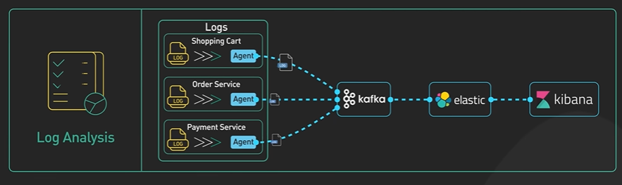
Real time machine learning techniques modern ml systems need to process vast data quickly and continuously, kafka makes it easy.
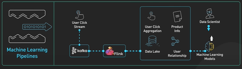
Example in a fraud detection system kafka streams transaction data to models. These models flags suspicious activities instantly. It might funnel sensitive data from amchine to model that forecast failures. Kafka integration with stream processing framework Flink or Spark streaming is key here.
These tools can read from Kafka write complex computation or ML inference and write results back to Kafka all in real time.
Kafka Stream is Kafka’s native stream processing library it allows us to build scalable, fault tolerance stream processing applications directly on top of Kafka.
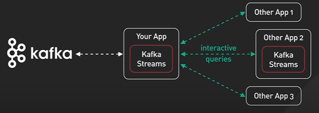
The 3rd use case is real time system monitoring and alerting - Log analysis helps investigate past events, it’s about immediate protective system health tracking and adverting.
Kafka ingest data from various source - application performance metrics, server health stats, network traffic data.
Data flows through Kafka and stream processing applications continuously analyse it, they can compute aggregates or trigger alerts all in real time.
Kafka Pub/Sub model shines here multiple specialised consumers can process the same stream of metrics without interfering with each other. One might update dashboards and other can manage alerts while 3rd to feed a machine learning model for predictive maintenance.
Kafka persistence model allows for time travel debugging we can replay the metric stream to understand the system state leading up to an incident. This feature can speed up with root cause analysis.
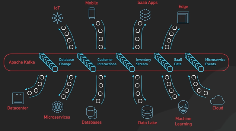
The Kafka use case involves change data capture cdc is a method used to track the capture changes in source databases it allows these changes to be replicated to other systems in real time.
Kafka acts as a streaming changes from source databases to various downstream systems.
The process begin with the source db and all change are added in the database and the databases generate transaction logs that records all data modifications such as inserts updates and delete in the order they occur.
The transaction log feeds into Kafka, it stores the change events in topics it’s allowed multiple consumers to read from them independently. This is where Kafka power as a scalable durable message broker comes into play.
To move data between Kafka and other systems we use Kafka connect.
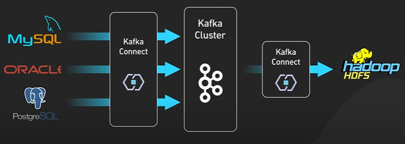
This framework allows us to build and run various connectors for instance we might have an elastic search connector to stream data to elastic search for powerful search capabilities and a db connector to replicate data to other databases for backup or sailing purposes.
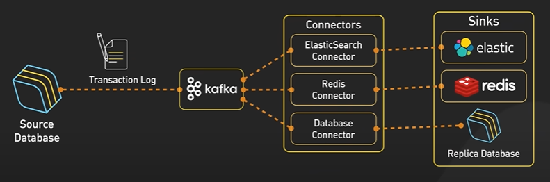
The 5th use case is system migration kaka does more than just transfer data in migration it acts as a buffer between old and new systems, can also translate between them this allows a gradual low risk migrations.
Kafka lets engineers implement complex migration patterns these include strangler fake and parallel run comparison.
Kafka can replay messages from any point in its retention period. It is a key for data reconciliation. It maintains consistency during the migration process. Kafka act as a safety net for large migration.
User can run old and new system simultaenously and bothe system can generate and consume data in kafka. It allows for easy rollback if issues arise.
Why Kubernetes popular.
Kubernetes is an open-source platform designed to automate the deployment, scaling, and management of containerized applications.
As applications have grown more complex, developers have started breaking them down into smaller, independent services. These microservices are typically packaged in containers, which provide an ideal environment for running them.
But here’s the catch: as applications scale up, managing all these containers manually becomes a nightmare.
It offers a streamlined approach to container orchestration. Kubernetes High Availability. Downtime is costly. Kubernetes helps our applications to remain accessible with minimal interruptions. It does this by automatically restarting failed containers, distributing load across multiple instances, and offering self-healing capabilities.
Scalability. As our user base grows, the applications need to handle increased load. Kubernetes makes it easy to scale our applications up or down in response to changing demand. This flexibility ensures optimal performance and resource utilization.
A typical Kubernetes cluster consists of the control plane and multiple worker nodes. The worker nodes are the workforses of the cluster. They’re responsible for running the containers that make up our applications.
The number of containers on each worker node depends on factors like resource requirements and overall workload distribution.
Each worker node runs a process called Kubelet, which acts as a local agent that enables communication and coordination within the cluster.
The control plane, on the other hand, serves as the command center. It orchestrates and manages the entire cluster.
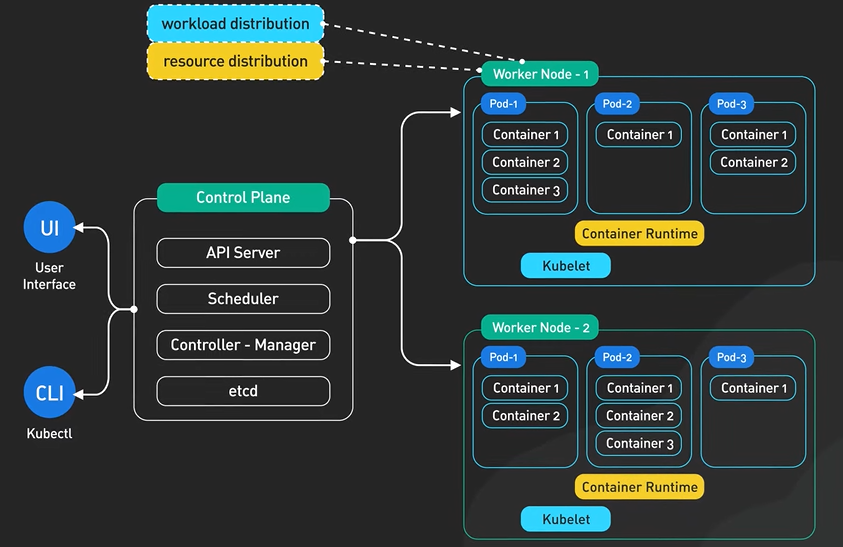
It runs several critical Kubernetes processes: First, there’s the API Server. Think of this as the central communication hub of the cluster. It’s the entry point for various Kubernetes clients, including user interfaces, APIs for automation, and command-line tools.
Next, we have the Controller Manager. This component maintains the desired state of the cluster. It continuously monitors the cluster’s health, identifies any deviations from the desired state, and takes corrective actions. Then there’s the Scheduler. It distributes incoming containers across the worker nodes based on resource availability and specific requirements.
Underpinning all of this is etcd. It’s a robust key-value store that serves as the persistent memory of the cluster. It securely stores all configuration data and the real-time status of each node and container.
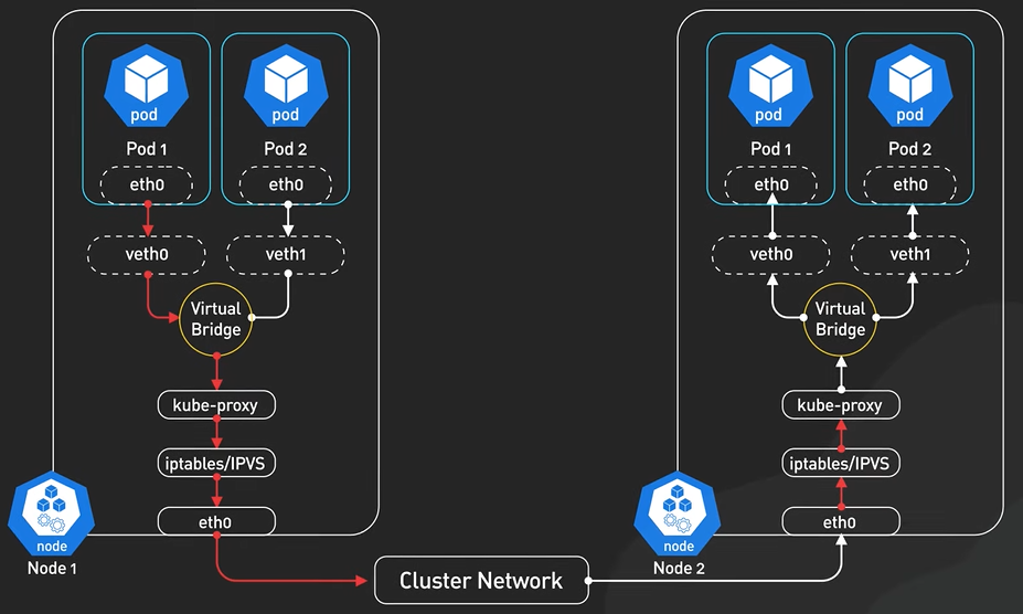
To enable seamless communication between nodes, Kubernetes uses a virtual network that interconnects all nodes within the cluster. This virtual network abstracts away the underlying physical infrastructure and presents the cluster as a unified computing resource.
In terms of resource allocation, worker nodes typically have more CPU, memory, and storage compared to control plane nodes. This is because they bear the brunt of the workload by running numerous application containers. Control plane nodes, while running fewer processes, are critical for cluster operation.
In production environments, it’s common to deploy multiple control planes for redundancy and fault tolerance.
A pod is the smallest deployable unit in Kubernetes. It is an abstraction layer on top of one or more containers that logically belong together.
In our web application scenario, we’d have an “application pod” hosting the web server and a “database pod” managing the database. Pods in Kubernetes are ephemeral.
If a pod fails or needs to be rescheduled, Kubernetes will automatically create a new one to replace it.
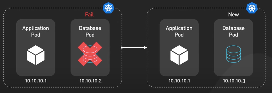
However, this new pod might have a different IP address, which can pose a challenge for inter-application communication.
To address this, Kubernetes introduces the concept of Services.
A Service provides a stable IP address and DNS name that acts as an internal load balancer for a group of pods. Even if individual pods are recreated, the service’s IP address remains constant, ensuring consistent communication.
For our web application to be accessible to users outside the cluster, we need to expose it to the internet.
Kubernetes offers External Services for this purpose. It opens up a specific port on the cluster’s network and routes incoming traffic to the appropriate backend pods.
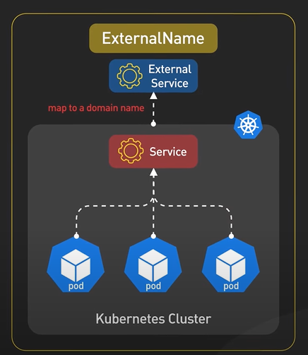
While External Services technically expose our application, the default URLs they provide can be complex and not very user-friendly.
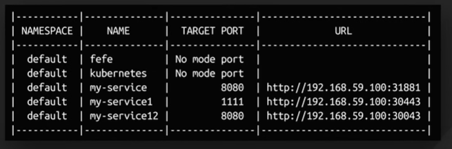
This is where Kubernetes Ingress comes into play. Ingress acts as a smart reverse proxy, allowing you to define rules for routing external traffic to specific services within the cluster based on the request’s URL.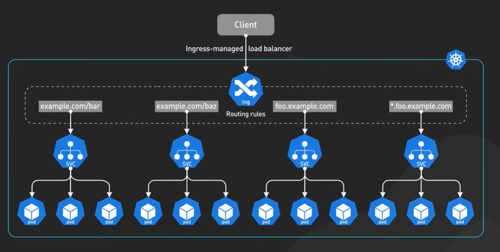
Kubernetes also provides mechanisms for managing application configuration data. ConfigMaps stores configuration data like database connection URLs or API endpoints, while Secrets stores confidential data like passwords and API keys.
Kubernetes offers two primary mechanisms for managing pod replicas: Deployments and StatefulSets.
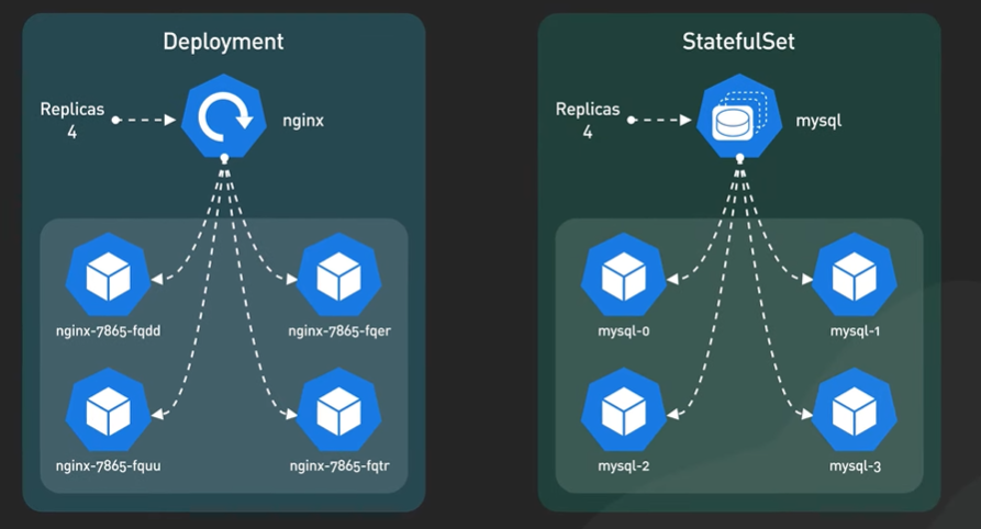
Deployments are ideal for stateless applications, like our web server, where each replica is interchangeable. We can define a Deployment that specifies the desired number of replicas for our application pod, and Kubernetes will ensure that number is always running.
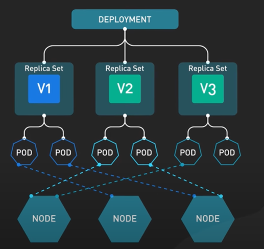
Data are safe and sound in Kubernetes. Kubernetes Volumes provides a mechanism for abstracting storage from the lifecycle of pods. It allows us to mount external storage directly into the pods. This is useful for scenarios where data needs to be persisted even if a pod is deleted and recreated.
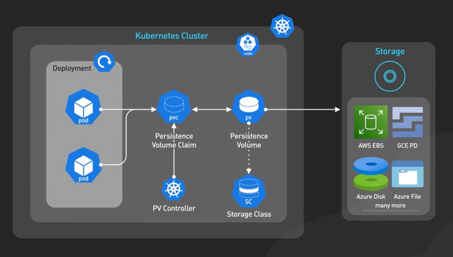
For stateful applications like databases, Kubernetes provides StatefulSets.
These build upon the functionality of Deployments but offer additional features tailored for applications that require persistent storage and careful management of data consistency across replicas.
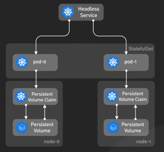
While StatefulSets offers a way to manage stateful applications like databases within Kubernetes, setting up and operating databases in Kubernetes can be complex and require specialized knowledge.
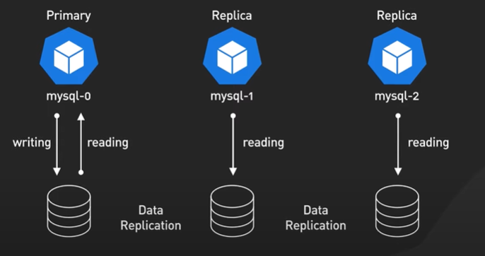
Many organizations opt for a hybrid approach. Instead of running databases directly in Kubernetes, they might host their databases externally, perhaps on dedicated database-as-a-service platforms. They then connect their applications running within Kubernetes to these external databases. This hybrid approach offers a balance.
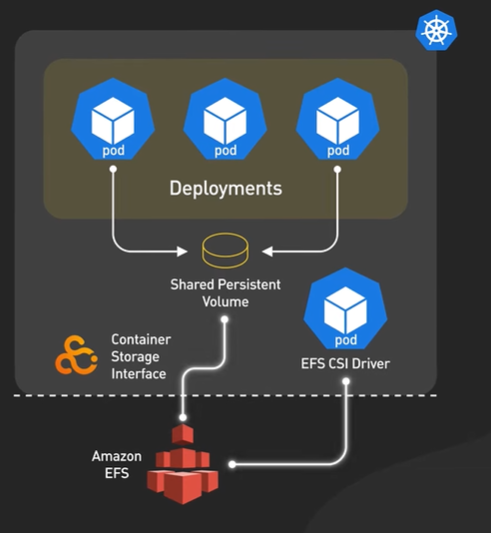
It allows organizations to leverage the benefits of container orchestration for their applications while avoiding the complexities of managing stateful applications like databases within the Kubernetes environment.
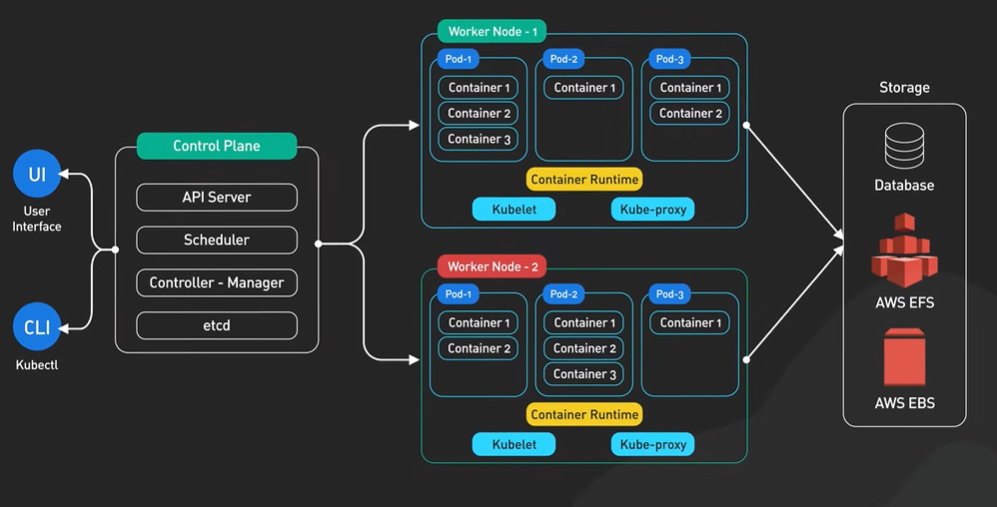
On the downside, complexity is the number one drawback. Kubernetes is complex to set up and operate. It comes with a high upfront cost, especially for organizations new to container orchestration. It requires a high level of expertise and resources to set up and manage a production environment. Cost is also a drawback, as Kubernetes requires a certain minimum level of resources to run in order to support all its features, likely making it overkill for many smaller organizations.
One popular option that strikes a reasonable balance is offloading the management of the control plane to a managed Kubernetes service, which cloud providers offer. Some popular ones are Amazon EKS, GKE on Google Cloud, and AKS on Azure. These services allow organizations to run Kubernetes applications without worrying about the underlying infrastructure.
Scalability Explained.
A system is scalable if it can handle increased loads by adding resources – without compromising performance. But there’s another layer to this: scalability isn’t just about handling more work; it’s about doing so efficiently. It’s about applying a cost-effective strategy to extend a system’s capacity.
This shifts our focus from merely surviving increased demand to optimizing how we scale.
One effective way to understand system scalability is by analyzing response vs. demand curves.
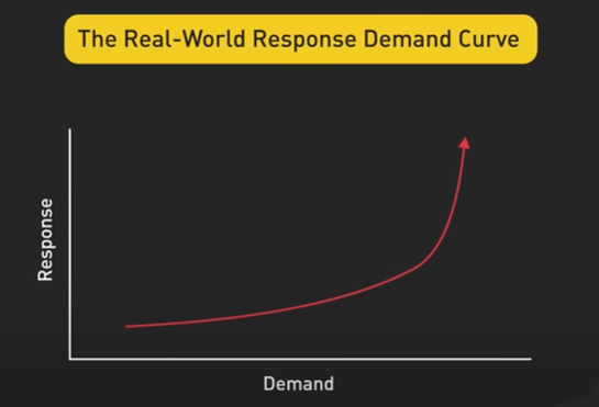
This tipping point when it start to increase often appears as a “knee” in the response vs. demand curve where performance starts to degrade rapidly. Our goal in system design is to push this knee as far to the right as possible, delaying that performance drop-off for as long as we can.
What typically causes scaling bottlenecks?
There are two main culprits. Centralized components and high latency operations.
A centralized component, like a single database server handling all transactions, creates a hard upper limit on how many requests our system can handle simultaneously.
High latency operations, such as time-consuming data processing tasks, can drag down the overall response time, no matter how many resources we throw at the problem.
However, sometimes centralized components are necessary due to business or technical constraints. In such cases, we need to find ways to mitigate their impact, such as optimizing their performance, implementing caching strategies, or using replication to distribute the load.
Building system scalable - Statelessness, loose coupling, asynchronous processing.
statelessness. This means our servers don’t hold onto client-specific data between requests. By keeping servers stateless, we make it easy to scale horizontally because any server can handle any request. Plus, it enhances fault tolerance since there’s no crucial state that could be lost if a server goes down. However, it’s important to note that some applications require maintaining state, such as user sessions in web applications. In these cases, we can externalize the state to a distributed cache or database. This allows the web servers to remain stateless while the state is preserved.
Next, loose coupling. This is all about designing systems components that can operate independently, with minimal dependencies on each other. By using well-defined interfaces or APIs for communication, we can modify or replace individual components without causing ripple effects throughout the system. This modularity is important for scalability because it allows us to scale specific parts of the system based on their unique demands. For example, if one microservice becomes a bottleneck, we can scale out just that service without affecting the rest of the system.
asynchronous processing. Instead of having services call each other directly and wait for a response, which can create bottlenecks, we use an event-driven architecture. Services communicate by emitting and listening for events, allowing for non-blocking operations and more flexible interactions.
Vertical scaling, or scaling up, involves increasing the capacity of a single machine. This could mean upgrading to a larger server with more CPU, RAM, or storage. It’s straightforward and can be effective for applications with specific requirements or when simplicity is a priority. For example, vertical scaling might be preferable for database systems that are challenging to distribute horizontally due to consistency constraints. However, vertical scaling has physical and economic limitations.
Horizontal scaling, or scaling out, involves adding more machines to share the workload. Instead of one super powerful server, we have multiple servers working in parallel. This approach is particularly effective for cloud-native applications and offers better fault tolerance.
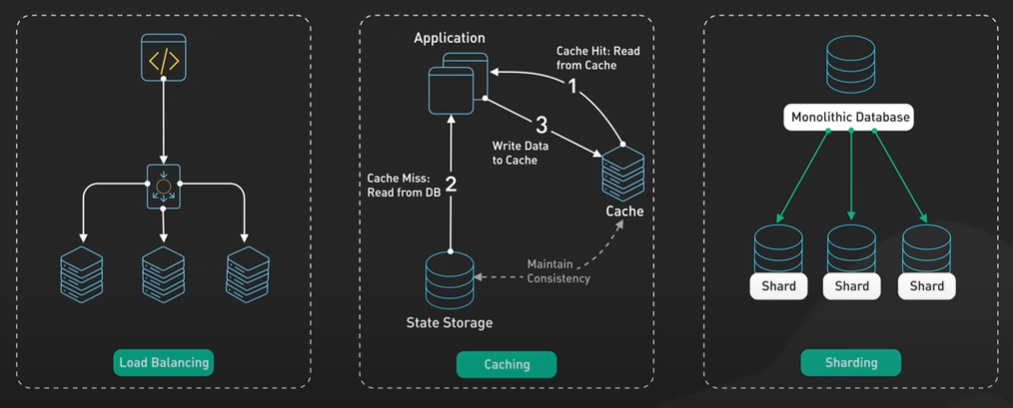
Sharding involves splitting large datasets into smaller, more manageable pieces, each stored on different servers. This allows for parallel data processing and distributing workload across multiple machines. The key is choosing the right sharding strategy and keys based on the data access patterns to ensure even distribution and minimal cross-shard queries.
A golden rule in scalability.
Avoid centralized resources whenever possible. Centralized components become bottlenecks under heavy load. Instead, think distributed. If we need a queue, consider using multiple queues to spread the processing load. For long-running tasks, break them into smaller, independent tasks that can be processed in parallel. Design patterns like fan-out, pipes, and filters can help distribute workloads effectively across our system. Finally, embrace modularity in system design. By creating loosely coupled, independent modules that communicate through well-defined interfaces or APIs, we enhance both scalability and maintainability. Keep a close eye on key metrics like CPU usage, memory consumption, network bandwidth, response times, and throughput.
Components of Web Applications.
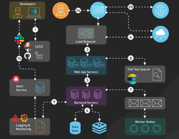
CICD pipelines the backbone of modern development tools like GitHub actions automate testing, building and deployment.
The path of a user request is starts in the browser after DNS resolution the request heads to our application servers but before it gets there it hits two critical components load balancers and reverse proxies.
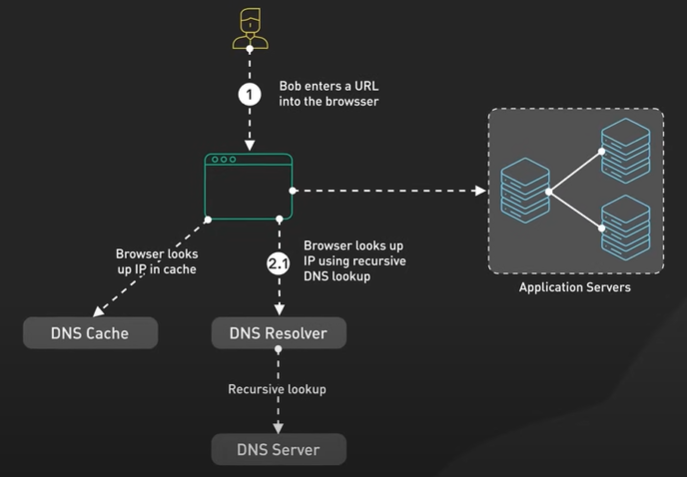
Content delivery networks or cdns these are distributed global serving static content like images and JavaScript closer to users the result faster load times.
We use distributed caches the redis keeping frequently accessed data in memory for speed.
In heavier tasks we use job workers not everything can be done in real time so for resource intensive or long running tasks job queues come in handy these tasks are offloaded to worker notes keeping it responsive.
if the app needs search functionality services like elastic search are invaluable they provide fast flexible large data sets helping user find what they need quickly.
Promethus, Grafana and DataDog help track everything logs, performance metrics and resource usage.
Finally when something does go wrong we need reliable alerting platforms that pagerDuty send realtime alerts to the team.
How SSH really works.
SSH create a secure tunnel between client and server.
SSH2 provides more secure than SSH1.
| SSH2 | SSH1 |
|---|---|
| Separate transport, authentication and connection protocols. | One monolithic protocol. |
| Strong cryptographic integrity check. | Weak CRC-32 integrity check. |
| No server keys needed due to Diffie Hellman Key exchange. | Server ey used for forward secrecy on the session key. |
| Supports public key certificates. | N/A. |
| Algorithms used - DSA, DH, SHA-1, MD5, 3DES, Blowfish, Twofish, CAST-128, IDEA, ARCFOUR. | RSA, MD5, CRC-32, 3DES, IDEA, ARCFOUR, DES. |
| Periodic replacement of session keys. | N/A. |
SSH client attempts to connect to a server it begins by establishing a TCP connection on port 22.
TCP connection is in place the client and server start version negotiation this step ensures both parties are speaking the same language agreeing on which version of the ssh protocol they will use for this session.
Next algorithm negotiation here the client is server decide which cryptographic algorithms there is used for key exchange encryption and integrity checking.
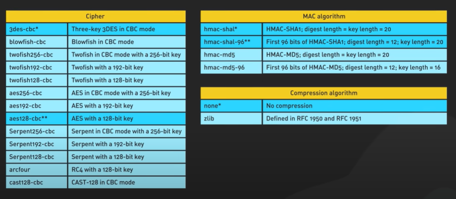
This negotiation allows ssh to adapt to different security requirements and computational capabilities
We reach a critical step in the SSH handshake Key Exchange.
The client and server using elliptic curve Diffie Hellman method to generate a shared certificate in this process both sides generate ephemeral key pairs and exchange their public key to dynamically create shared secret for encryption.
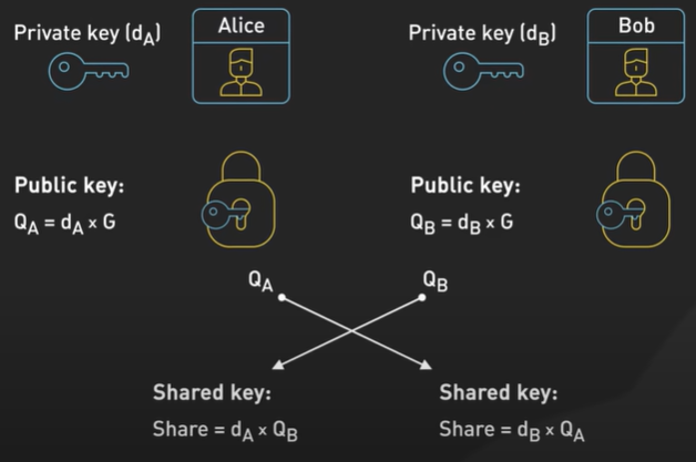
The use of ephemeral keys provides perfect for secrecy meaning that even if the keys are compromised in the future pass session data were being secured.
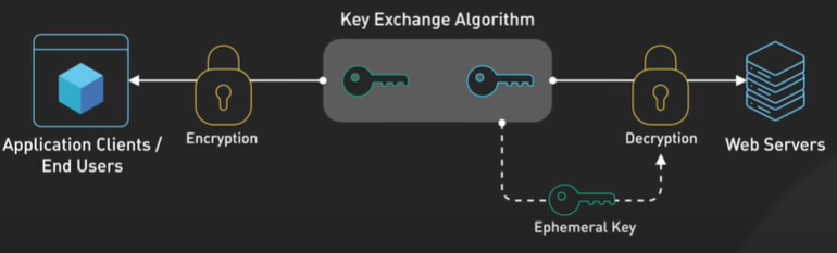
The shares secret key is then used for symmetric encryption which encrypts all the data transmitted during the ssh session.
Now their client initiates a login request to the server the server then performs a critical security cheque by looking at a matching public key in its authorised key files typically located in .ssh authorised keys on Unix file systems.
This method known as public key authentication is the most common way to verify their clients is allowed to connect to the server. SSH also support password based authentication although it’s less secure compared to public key authentication.
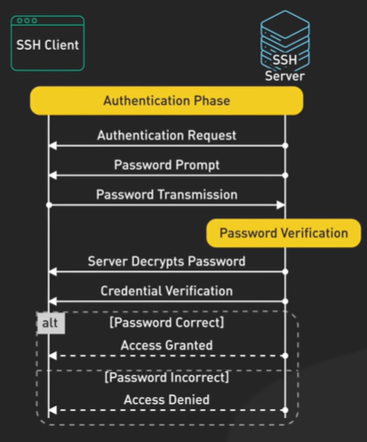
If the server finds a matching key it encrypts a random number using the client’s public key and sends it back to the client.
This challenge serves two purposes improves that the server has the correct public key and ensures that the client processes the corresponding private key.
The client that decrypts this random number using his private key but successfully decrypting the data and sending it back to the server the client proves his identity.
The server verifies the decryption confirming that the client is who it claims to be.
Once the authentication is complete the SSH session is fully established from this point on all commands sent from the client to the server encrypted with the session key.
The server executes these commands and cribs the result using the same session key and sends them back to the client.
The client then decrypts this result using the session key this encrypted back and forth continues for the duration of the SST session.
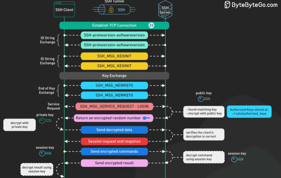
SSH local forwarding which allows you to turn no other network services through the ssh connection this can be especially useful for accessing services that might otherwise be blocked by Firewalls or for adding a layer of security to an encrypted protocols.
Big O Notation.
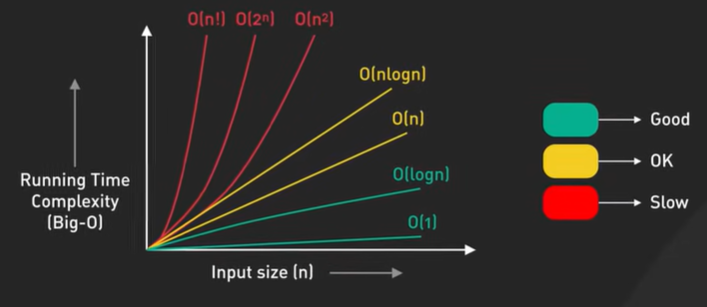

The real world performance can differ due to caching, memory usage and hardware specifics.
With modern CPU maximizing the cash hit can sometimes be much more beneficial than optimizing the algorithm.
In a traversal the row by row is often faster than column by column. Row access maximize the sequential access and is cache friendly.
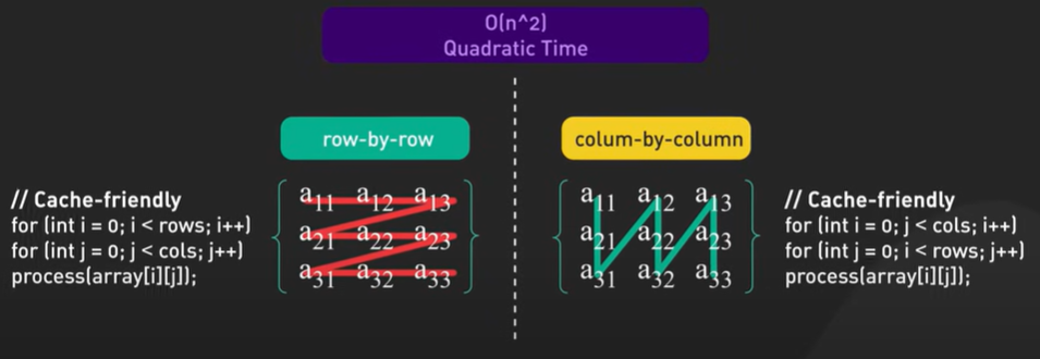
API Paginations.
Pagination is a way to split the result into pieces and let client request them one at a time.
Instead of sending thousands of records at a time we sent them in batches of 10 or 100. It helps in the server load and reduces traffic and keeps our application more responsive.
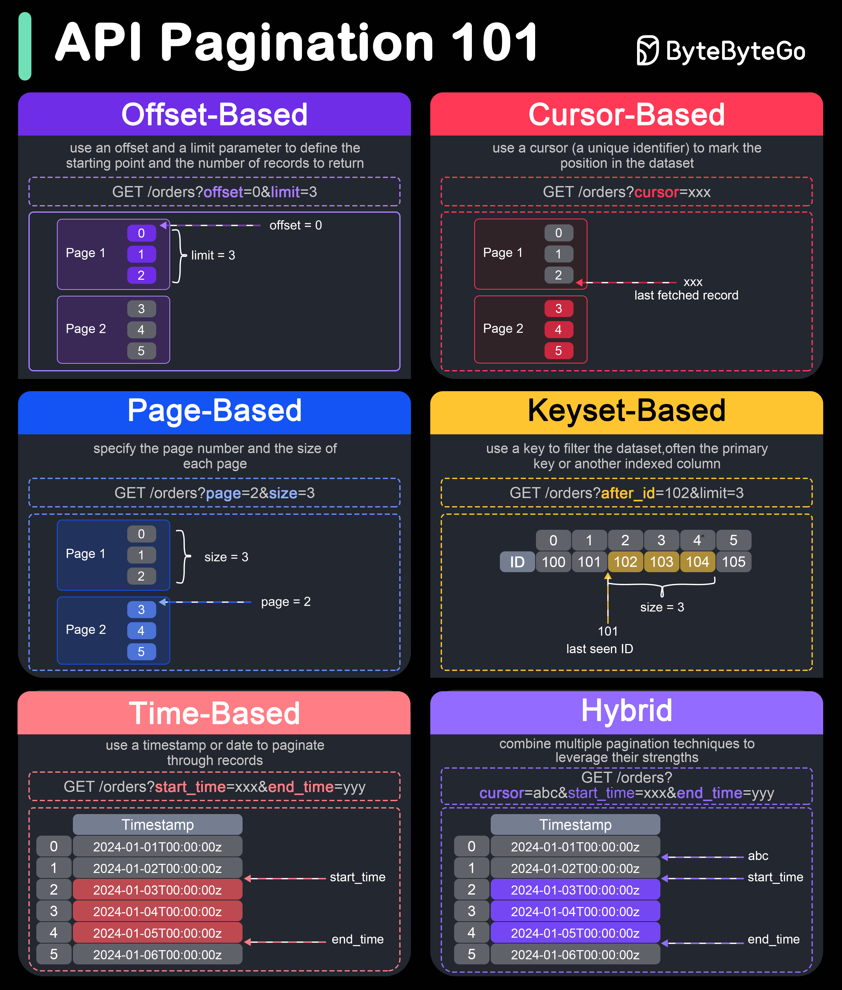
There are two main ways to handle pagination offset based and cursor based.
Offset based pagination has 2 forms - Page based and direct offset based.
Page based set how many item we want per page then calculate where to start.
Direct offset use the offset and limit parameters directly. Basic offset query looks like SELECT * FROM table LIMIT 10 OFFSET 20;
Offset based pagination is easy to build but it has problem with large datasets.
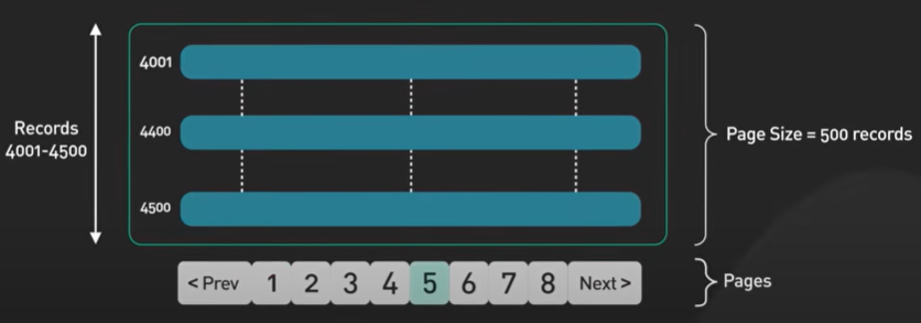
The database has to process every row to the offset before it can return results.
There is another problem when database changes fast then the offset based pagination can miss record or show them same data again the new data added will shift the data around.
Cursor based offset fixed the problem.
First pick an index column like an id as cursor then hash the cursor value for security.
Client sends their last scene cursor value. We use this cursor to filter and fetch the next batch. Send the result and new cursor for the last item. Client uses the new cursor for the next request.
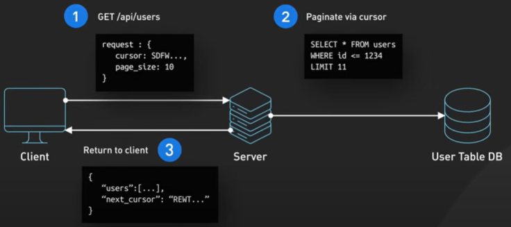
Cursor based pagination works really well with large data set as it stays consistent even when new records are added or deleted in between request. It is perfect for some real time feeds or any data that changes often.
Some cursor based implementation are Keyset-based pagination and Time based pagination.
Keyset pagination uses index keys such as primary key to retrieve the next set of result by directly accessing rows without scanning preceding ones.
Time based pagination uses timestamp as cursor to segment and retrieve the data within specific time ranges.
Cursor based methods for large and fast changing data set.
Apache Kafka Fundamentals.
Kafka is a distributed event store in real time streaming platform it was initially developed at LinkedIn and has become the foundation for data heavy applications.
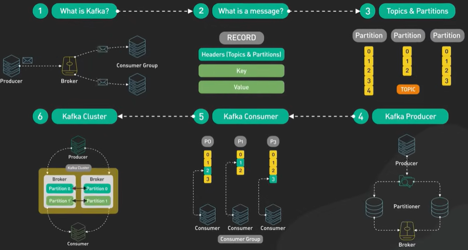
Every piece of data Kafka handles is a message.
Kafka messages three parts - headers which carry metadata, the key which helps the organization and the value which is the actual deploy payload.
Topic and Partition - Kafka organizes the messages using the topic and partitions. The structure the data streams within each topic goes a step further by dividing it into partitions. These partitions are key to Kafka scalability because they allow messages to be processed in parallel across multiple consumers to achieve high throughput.
Multiple consumers to achieve high pumping capital cross
Why most company uses Kafka?
Kafka is creating a handling multiple producers sending data simultaneously without performance degradation. It also handles multiple consumers efficiently by allowing different consumer groups to read from the same topic independently.
Kafka tracks was being consumed using consumer offset store with the counter itself this ensures that consumers can resume processing for where they left on the case of failure.
On top of that Kafka provides this space retention policies to allow us to store messages even after they’ve been consumed based on time or size limits we define nothing is lost unless we decide it’s time to clear it.
Kafka scalability means we can start small and grow as the needs expand.
Producers - Applications that create and send messages to Kafka. Producers batch messages together to cut down a network traffic they use partitioners to determine which partition a message should go. No key is provided messages are distributed randomly across partitions if a key is present messages with the same key are sent to the same partition for better distribution.
On the receiving end we have consumers and consumer groups. Consumers within a group share responsibility for processing messages from different partitions in parallel. Each partition is assigned to only one consumer within a group at any given time. If one consumer fails another automatically takes over its workload to ensure an uninterrupted processing.
Consumers in a group divide up partitions among themselves through coordination by Kafka’s group coordinator.
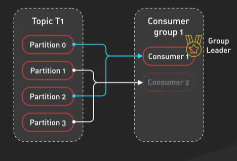
When a consumer joins or leaves the group calculus triggers a rebalance to redistribute partitions among the remaining consumers.
The Kafka cluster itself is made up of multiple brokers. This server store and manage of data to keep a data safe each partition is replicated across several brokers using a leader follower model.
If one broker fails another one steps in as new leader without losing any data.
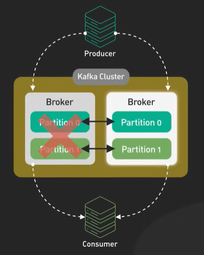
In earlier versions Kafka relies on zookeeper to manage broker metadata and leader election.
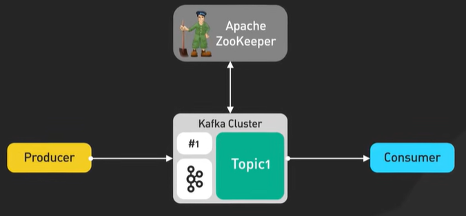
Newer versions are transitioning to craft a building consensus mechanism that simplifies operations by eliminating zookeeper as an external dependency while improving scalability.
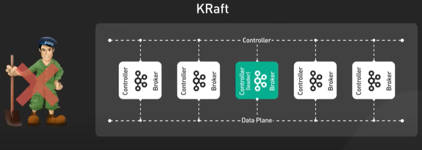
Kafka in real application.
It’s widely used for log aggregation for thousands of servers.
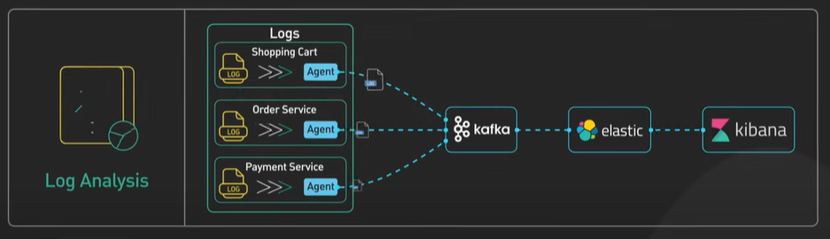
The most chosen for real time events streaming for various sources.
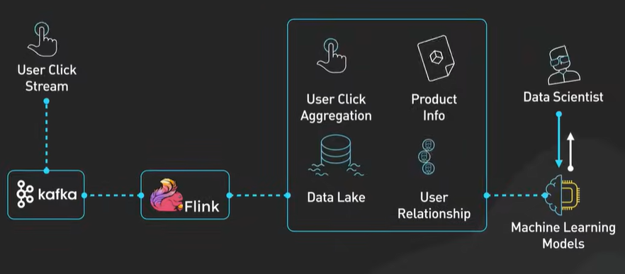
Change data capture it keeps database synchronize across systems.
It is invaluable for system monitoring by collecting metrics for dashboards and alerts across industries by finance healthcare retail and IOT.
Most important system design concepts.
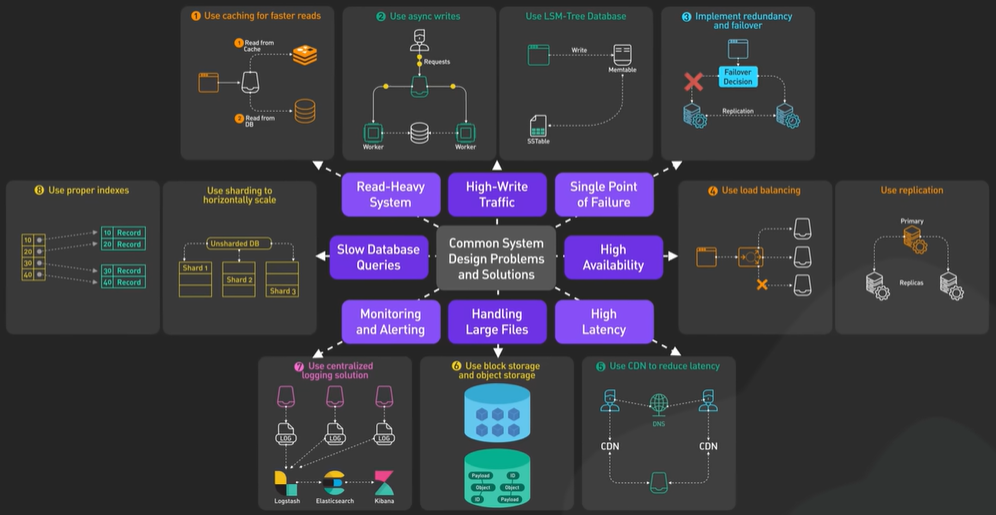
Read Heavy System - Use cache.
Write Heavy - Logging System processing millions of events per second, social media handling users interactions.
Managed in two different ways - Asynchronous write with message queue, LSM Tree based database like Cassandra.
These databases collect writes in memory and periodically flushes them to disk as sorted files. To maintain performance they perform compaction merging files to reduce the number of lookups required during reads. It make the write fast and the read slower as it see multiple files.
System with single database server is a fail. It solved with redundancy and failover. Implementing database replication with primary replica instances. It increases availability but introduces a complexity in consistency management. We must use synchronous replication to prevent data loss and accept higher latency.
Synchronize application to avoid data loss or asynchronous application to improve the performance with a slight risk to lose data during failures.
Some systems even use quorum based replication to balance consistency and availability.
Critical system like payment requires high availability and that may need load balancing and replication together.
Load balancer distribute traffic across surf cluster and read out during failure. Primary replica setup is standard the primary handles the write and the multiple replica handles the read. Failover ensures a replica becomes the leader and become the primary.
Multiple primary replication is another option for distributed write geographically.
Performance becomes critical when serving users globally. In America user should not wait to load the data from servers in Europe. CDN solves this by caching content closer to user and dramatically reduces the latency.
Static content like videos and images are perfectly with CDN’s. For dynamic content solutions like edge computing can complement CDN cache.
Different types of content need different cache control headers longer duration for media files, shorter for user profiles.
Managing large amount of data brings its own challenges modern platform use two different type of storage block storage and object storage.
Block storage with its low latency and high IOPS is ideal for databases and frequently accessed small files.
Object stories on the other hand cost less and is designed to handle large statistics videos in backup at scale.
Most platform combines these user data goes into block storage and media files are stored into the object storage.
Modern monitoring system like Prometheus collects the log and metrics and Grafana provides a visualization.
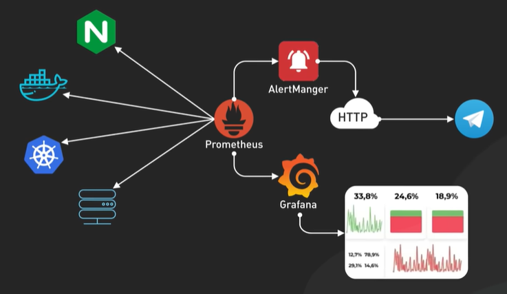
Distributed tracing tools like OpenTelemetry helps debug performance bottle neck across components.
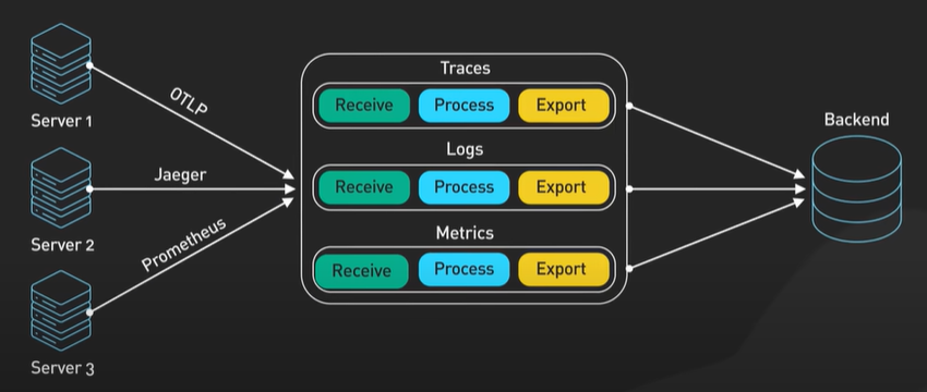
At scale managing this flood update is challenging.
The key is to sample routine events keep detailed logs for critical operations and setup alerts that trigger only for real problems.
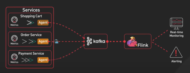
The most common issue is monitoring reveals his slow database queries.
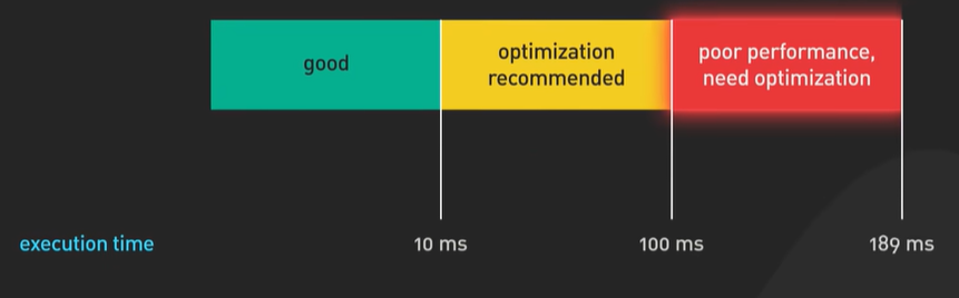
Indexing is the first line of defense.
Without indexes the database scans every record to find what it needs with index it can quickly jump to the right data.
Composite index for multi column queries can further optimise performance.
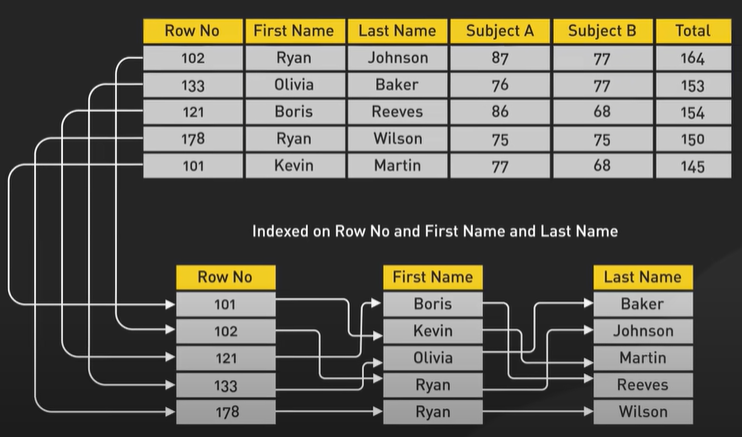
Every index slow down the write slightly since they need to update as data changes.
Sharding splitting the data in to multiple machines using strategies like range based or hash based distribution.
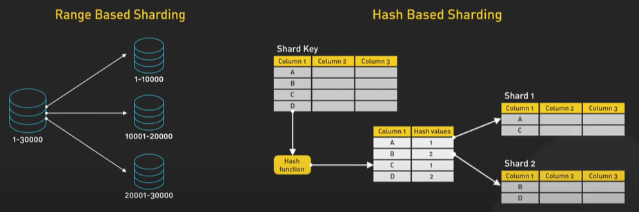
API vs SDK.
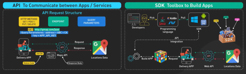
API - Application programming interfaces are universal translators they let different software applications talk to each other instead of building everything from scratch
API use REST architecture in a way of communicating through http requests.
SDK - Software Development Kits APIs are the raw connection points between services SDK are like prebuilt toolboxes that make those connection easier to use they handle the complex technical details so we can focus on building features.
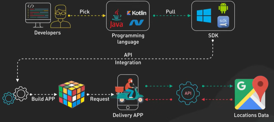
SDK is a complete package it comes with tools, libraries and documentation everything we need to build apps with specific platforms Android or IOS.
A well designed SDK takes all those platform complexities and simplifies them making sure our apps behave consistently across different devices many.
SDK come with pre built api clients that make integration easy these clients handle all the technical heavy lifting they manage authentication, they format request properly, they try complicated responses into data that’s easy to use in our code.
Instagram’s SDK instead of writing hundreds of lines of code to connect with Instagram’s api the SDK lets us add a shared Instagram feature with minimal effort.
When should we choose between an API and SDK?
Direct api integration makes sense when we need complete control over our project it’s a good choice when we want to keep our dependencies minimal and sometimes we might be working with a platform that doesn’t have an SDK that’s when APIs become our best friend.
SDKs take a different approach they’re fantastic when we need to move fast and get a product to market quickly they come back with best practices built right and if we need special features for specific platforms SDKs are often the way to go.
Many successful apps use both SDKs for their main use cases and direct api access for custom features.
Together these tools form the building blocks of modern software development.
What is Load Balancer.
Load Balancer is a software component that distributes the network and the application traffic across multiple servers.
It helps distribute the workload preventing any single server becoming the bottleneck.
It enables to scale the application dynamically add and remove server as needed.
It reduce latency and improves response time.
Distributing the request across multiple server enhances availability by providing redundancy and failover option.
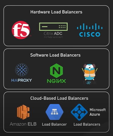
Hardware Load Balancer - High demand enterprise environments in dedicated data centers.
Load Balancer can also be classified by the network layer in which they operate.
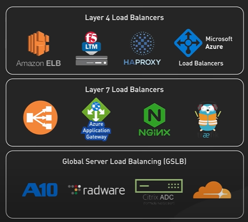
Layer 4 load balancer operate at the transport layer. It take the routing decision based on the IP addresses ports and TCP or UDP. They don’t consider the content of the request so it is faster. It is used for simplicity and efficiency.
Layer 7 load balancer operates at the Application layer at the HTTP and HTTPs. It enables the routing decision based on the content of the topic and content based routing. It can perform the SSL termination at the load balancer itself improving performance by offloading encryption and decryption from backend servers and centralizing SSL certificate management.
Global Server Load Balancing operate at higher level enabling traffic distribution across multiple location. GSLB consider the factor like user proximity to data center and the health of the backend infrastructure across the globe. They can use DNS based routing or any cast routing to direct the user to the nearest available data center.
Load balance to distribute the traffic using any of this selected algorithms.
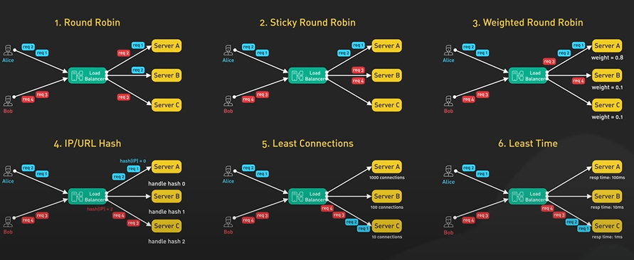
Load balance distribution algorithm.
Sticky Round Robin ties a client to a specific server by creating a session ID.
Weighted load balancer meaning assigning a weight to the particular server allowing the load balancing to send proportionately high number of requests to the capable server.
IP URL Hash where it is a bit different from the session round Robin where it will use a hash and redirect all the same ip route to the same server.
Why is Docker important.
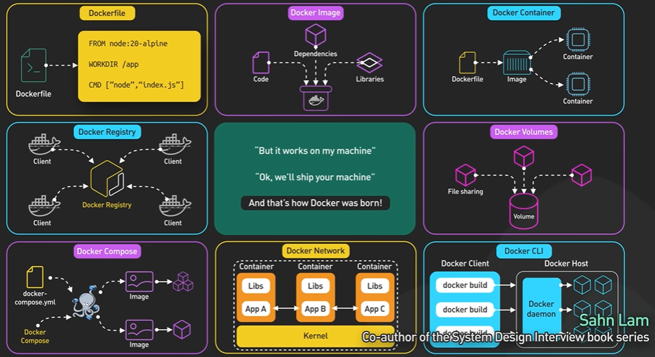
DockerFile - Defines the environment the application needs. It specify the base image and selecting only what is needed.
Get the light version and combine commands to reduce layers and remove build tools after compilations.
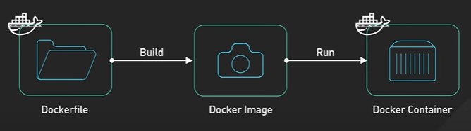
Inside the docker file each instruction creates a new layer and capture specific change in the file and configuration.
Specify te base image.
Install the dependency.
Copy the code.
Docker images are immutable once build cannot be modified. It is only replaced by new image. The immutability guarantee the software runs in production runs the same in testing.
Containers- The runtime instances of the image are light weight and shares the whole system kernel. Each container maintains a straight isolation through Linux kernel.

Namespace partition system resources that process network interfaces.
Cgroups provides fine grained resource control.
Multiple containers can run from a same image each with its own isolated state.
Distribution managed by Docker Registry. These repositories becomes the single source of truth for our images. Example DockerHub.
Data persistency in the container - Docker Volumes.
Unlike containers writable layers volumes exists independently and persist data across container life cycle.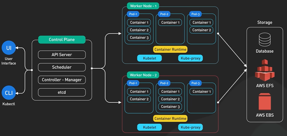
ContainerD and PodMan offer runtime focus on container execution and image management.
How Garbage collector works - Java, Python, Go.
The garbage collection mainly use the simple question like which object in the memory the program still use. It is answered through the concept of Reachability.
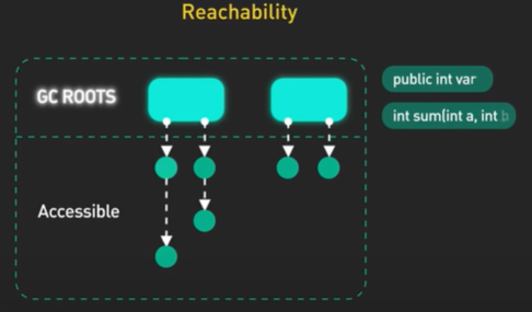
Every program has GC roots and these are the starting points like Global variables public int var and stack references int sum(int a, int b).
Any object that can be reached by following references from these roots is considered alive. Anything other than these are garbage.
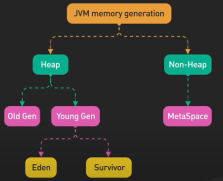
To efficiently manage the memory garbage collector Typically implement a generational hierarchy.

This design is based on empirical observation.
In java virtual machine is divided into 3 main areas - Young generation, old generation and meta space.
New objects start the life of the young generation Eden space If they survive multiple collections space they come to the survivor space in the Young generation.
The rare objects that persist even longer on the promotion to the old generation where collection happens less frequently but more thoroughly. The metaspace Java specific use class metadata to help reduce memory footprint in large application.
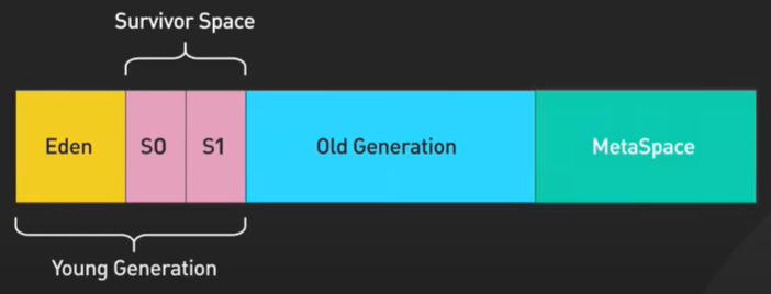
Other languages uses each generational collection differently. V8 users for two generation system and .NET Garbage collector typically uses three generation system.
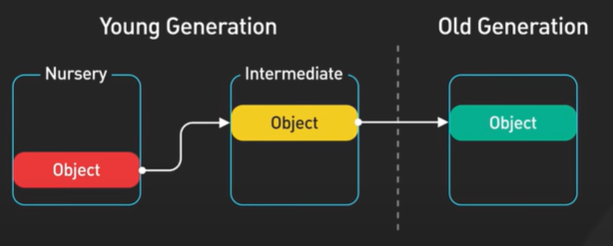
The most fundamental garbage collector strategy is the Mark and Sweep algorithm.
It happens in two phases it starts from the marked phase where it traverse all the references starting from the GC root marking each reachable object. In the sweep phase it reclaims memory from any unmarked object.
While effective this basic approach requires the application to completely pause during collection know as stop the world pause which can freeze the application for noticeable period of time.
The boss became more problematic when the heap size grows and application demands better responsiveness.
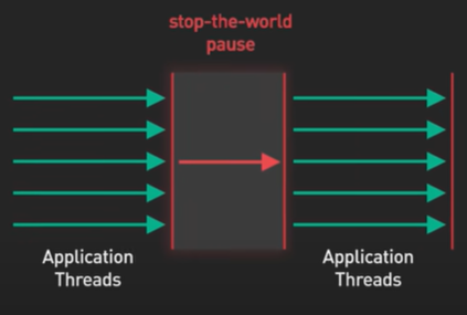
An advanced version is the Tri Color Mark and Sweep algorithm reduces the process by categorizing objects into three sets.
White Object are potential garbage.
Grey object are known to be reachable but have not been fully explored.
Black object are both reachable and fully processed.
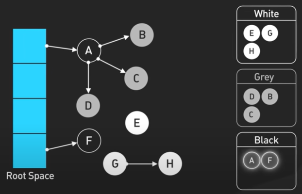
By maintaining these 3 distinct state the garbage collector can pause briefly to do initial marking then continuing examining grey object and their references while the application runs.
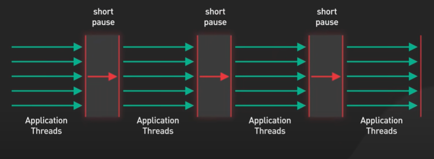
This incremental approach avoids the long pause required by traditional mark and sweep where the entire object graph must be traced at once.
Java offers several GC algorithms - Serial, Parallel, CMS, G1 Heap Allocation.
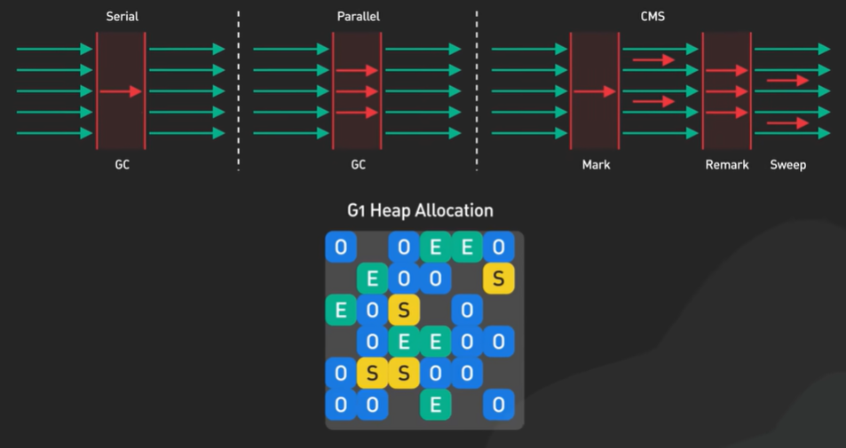
Python uses a combination of reference counting and a cyclic garbage collector.
The reference counting handles most cases By automatically de allocating objects when their reference drops to 0.
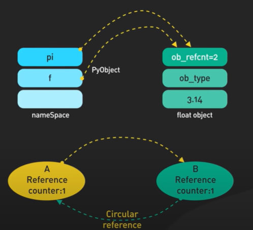
The cyclic collector cleans up circular references which the reference counting can manage.
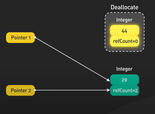
Go uses a concurrent mark and sweep collector which Operates alongside the application to minimise pause times.
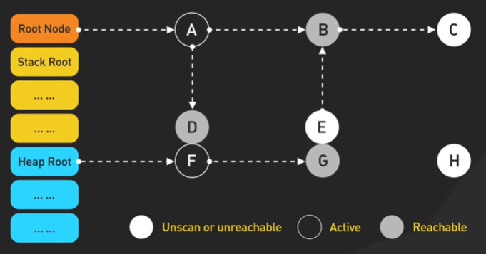
It uses the tricolor algorithm to handle the reachability.
GC Drawback - Performance overhead and Memory Fragmentation.
GC can produce long pause which does not matter for many application but can cause an issue in latency sensitive systems.
Some collectors leave gap in memory making allocation slower over time.
Memory management also involves balancing used pool and free pools to ensure efficient allocation and deallocation without fragmentation.
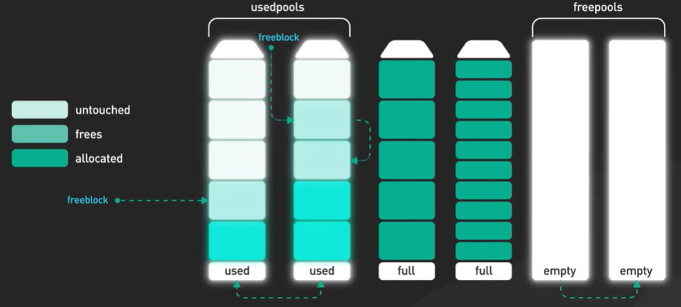
With garbage collection we usually lose fine grain controller over when clean up happens and it can lead to long pause.
Tips for designing fault tolerant systems.
Tips for designing Fault Tolerant System - Replication, Redundant, Fail Over, Load Balancing, Graceful degradation, Monitoring.
Fault Tolerant meaning system continues to function even when some component fails.
Replication - Each data is stored in several nodes. Cassandra replicates the data into multiple cluster.
Redundancy - Additional component that can take over in case of failure. Active active set up and both component running and load balancer distributing traffic between the component. Active passive set up a backup instance is ready and only works when there is one failure. Storage system like RAID also follow redundancy. RAID 0 split data across disks for performance but offers no redundancy. RAID 1 mirrors the same data across multiple disks and follow redundancy.
System monitor the data and when any failure detected the system redirect the data to the standby server.
Load Balancer to distribute the request to multiple server to avoid the crash of one server. NGINX and HAProxy are some of the famous load balancer.
Even with the strategies there will some failure or the recover takes longer than expected this is where the graceful degradation comes in. Instead of making the entire system stop graceful degradation ensures the most critical feature keeps still functioning.
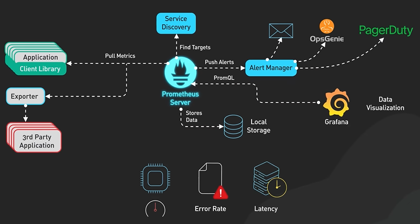
PagerDuty send the alerts any monitoring change.
Most popular open source AI stack.
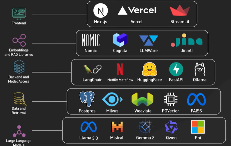
RAG - Retrieval-Augmented Generation.
What are AI Agents.
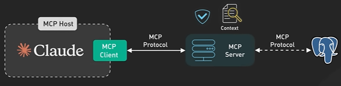
AI Agent is a helpful software assistance that can monitor what is happening around it and take smart action and acheive goals.
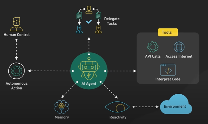
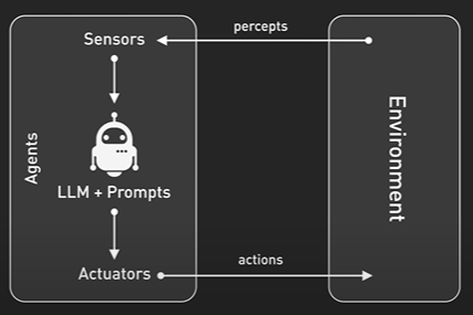
Different from traditional software. - Traditional system follows predetermined execution tasks.
Agents actively monitor their environment through inputs and sensors.
Process information through reasoning engines make decisions based on goals and available actions.
Take actions that modify their envirment and learn from feedback to improve performance.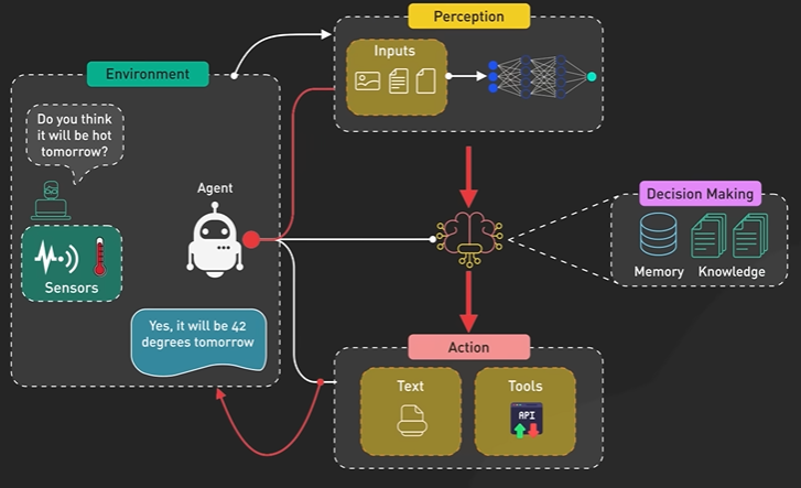
MCP - Model Context Protocol.
MCP is one of the most significant investments in LLM integration released by Anthropic in late 2024.
MCP is an open standard that enables Seamless integration between AI models and cloud and external data sources of tools.
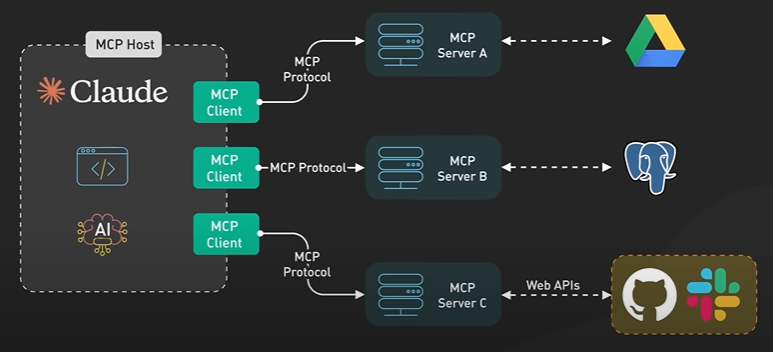
Before mcp connecting models to each new data source require custom implementations which can get expensive.
MCP solve this by providing a universal open centre for connecting ai systems with data sources replacing fragmented integrations with a single protocol.
It means we can give ai systems access to databases file systems apis and other tools in a standardised way.
The architecture mcp follows a client server models with 3 key components hosts, clients and servers.
Host are LLM applications like Clause desktop that provide their environment for connections.
Clients are components within the host that establish and maintain 1 to 1 connections with external servers.
Servers are separate processes that provide context, tools and prompts to these kinds exposing specific capabilities to the standardised protocol.
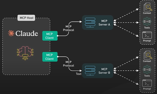
5 core primitive that powers MCP.
Resources structured data objects that can be included in the LMS context window they allow the model to reference external information.
Tools executable functions that the LLM can call to retrieve information or perform actions outside its context by querying a database or modifying a file.
In the client side they are two primitive they are equally important - Root primitive creating a secure channel for file access it allows the ai application to safely work with files on your local system by opening documents reading code or analysing data files without giving any restricted access to your entire file system.
Sampling primitive this enables a server to request a LLM when needed. Example when MCP is analysing the db schema it needs to generate query it can ask LLM to help formulating query through the sampling primitive.
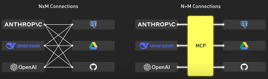
MCP one protocol and LLM vendors implement same protocol simplifies the integration.
Example - Using Claude to analyze data in the postgress db no need to build custom integration, use MCP server for Postgress that exposes db connection through the protocols primitive. Clause with the MCP client can query the db where the MCP server process the result and incorporate insights into the responses.
System Design Tradeoffs - Part 1, 2.
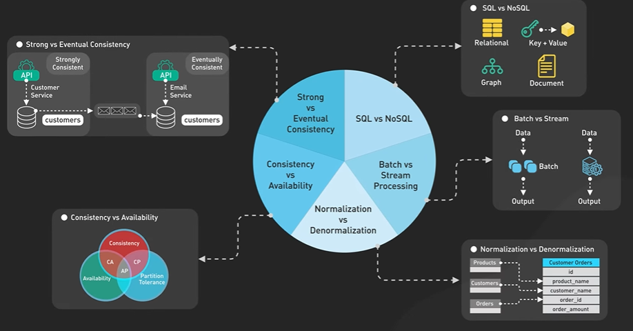
The application needs to prioritize and pick the correct trade offs.
Database - SQL strong consistency, structure schema, query capabilities. It creates issue in the horizontal scaling and scalability.
NoSQL solve the scaling issue and not maintain the consistency and structure.
In SQL all data are stored in different table to reduce redundancy. Application gets more data the cost of joins becomes more difficult and then denormalization comes into the picture. Normalization optimizes for the data integrity and storage and demoralization optimizes the read and cost of complexity in the query.
CAP - Strong consistency and Eventual consistency.
Data Processing - There are Batch Processing and Streaming.
Batch processing store the data and process at one go. It handles the computational efficiency and simpler error handling. There is latency and user needs to wait to get the insights.
Stream processing handles the data in real time as it arrives providing immediate results and enabling instant reaction to events.
The tradeoff here is the efficiency and simplicity vs the immediate and responsiveness.
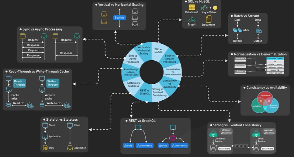
Vertical scaling increasing the power of the server. Horizontal scaling meaning increasing the number of server.
Stateful and Stateless - Game server needs to track the gamers position and need the state. Websocket server maintains persistent connections for chat applications. Trading platforms must track the session state for transaction. In these cases the stateful server is needed.
Modern architecture make stateless service for general application and stateful component for real time features.
Cache - Read-through and write-through.
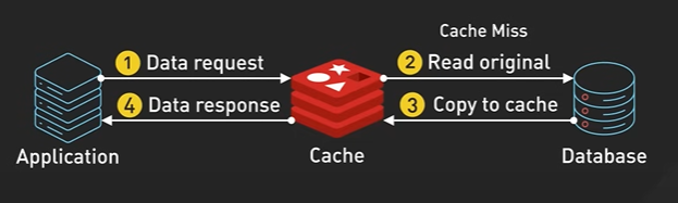
Read-through cache.
Read-through cache when the read is good. When there is new data then the write through cache needed.
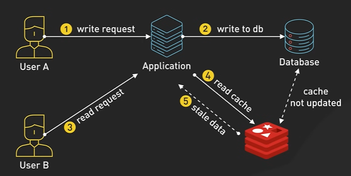
Write-through cache.
User A update the change and User B will request the data then there can be inconsistency in the data. The inventory system, booking system the data is important.
Write through cache update it by using both the db and cache.
API explained - 19th May 2025 completed.
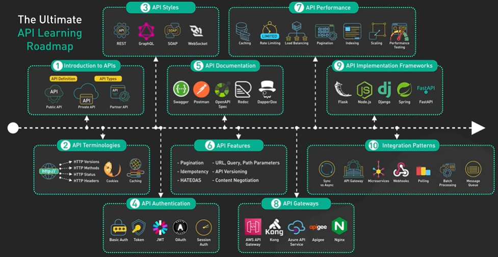
Application Programming Interface is a set of rules that allows system to communicate with each other.
There are 3 main types of APIs to know - Public API and Private APIs and Partner APIs.
Public API are open to anyone like Twitter or weather services.
Private APIs are connected internally within organization to connect with their systems.
Partner APIs are shared only with specific person who have the credentials.
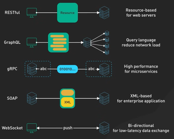
Video - API Protocol.
Http Status.
200 level - Success.
400 level - Something wrong with our request.
500 level - Something wrong at the server level.
Http Header and Cookies - Provide additional context and maintain the state across request.
Security.
Basic Auth - username and password.
Token Based Authentication - It provides temporary access tokens that can be revoked.
JWT - Json Web Token - It include digitally signed encoded user data within the token itself.
OAuth - It is standard for dedicated authorization across services.
Session Based Authentication - It is used in traditional web application by maintaining user state on the server.
API Documentation Tools.

Swagger and OpenAPI Specs are the online tool to make the documentation.
API Features involves - Pagination, Idempotency, URL Query Path Parameters, API versioning. It enhance visibility and resilience.
API Performance.
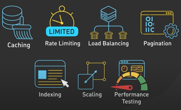
Caching to reduce server load and improves response time.
Rate Limiting - To protect against abuse.
Database index improves query performance for accessed data.
API Gateway services is the centralized entry point for managing all API traffic.
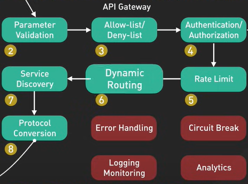
They handle request routing, authentication, rate limiting and monitoring.
Popular options of API Gateway.
AWS API Gateway - Cloud Native applications.
Kong - Open source flexibility.
Apigee - Enterprise grade API management.
API Integrations.
Webhooks - Event driven Integrations.
Batch Processing - large data volumes.
Message queue - Ensure delivery between system.
Trillions of Page - Google store the Page.
Patterns that enable high scale systems to handle massive data volumes efficiently.
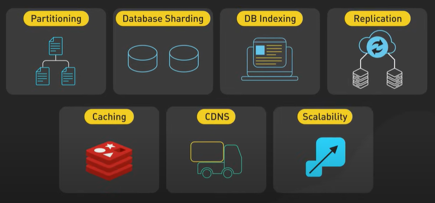
Data partitioning - Data partitioning divides data set into smaller more manageable segments. There are mainly 2 approaches for data partitioning - Vertical partitioning and Horizontal Partitioning.
Vertical Partitioning splits table by column based on access pattern and data characteristics. Most access hot data to be stored separately from rarely accessed cold data. Large text fields and binary objects can be segregated from structured data to optimize storage IO pattern.
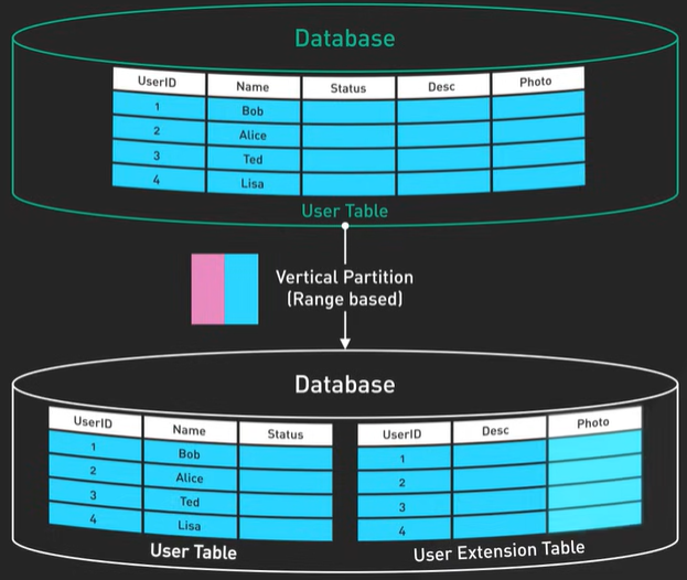
For example user table can store basic information in one partition and large biography text in another partition.
Horizontal partitioning - Horizontal Partitioning divides table by lose typically using a partition key to determine which row belong in which partition. Works well when data can be cleanly divided based on specific attributes such as price range or geographic regions.
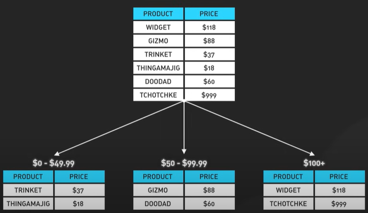
For example transaction table can be partitioned by month allowing queries for specific time period to access only relevant partitions.
Database sharding - Database sharding extends horizontal partitioning to distribute data across multiple independent database instances or server.
Partitioning generally happens on a single database and sharding spans across multiple database often separate physical machines.
Sharding distributes data using partition key and sharding strategies.
Hash based sharding applies a hash function to the shard key distributing data evenly but making range queries inefficient.
Range base sharding assigns rows to shards based on key ranges which optimizes for range queries but can create hotspot.
Directory based sharing uses a lookup service to map keys to shards. Flexibility and a added cost of additional complexity.
Major platform handles sharding to handle massive data volumes and write loads that can overwhelm a single database instance.
Database indexing creates auxiliary data structure that optimizes inquiry pattern at the expense of additional storage and right overhead. Modern Db implement various index types.
BTree index - BTree index are balanced tree maintenance stored data for range queries and point lookups.
Hash index - Hash index is provided direct key to location lookups but no range query support.
Bitmap indexes - Bitmap indexes are efficient for low cardinality column like boolean flags or status codes.
Inverted index - Inverted index map content to records. Provide full text search capabilities. Placed index can transform a full table scan taking minutes into AB3 traversal completing in milliseconds.
Each additional index imposes some right overhead as the database must maintain the structures during inserts and updates. This is one of the trade off in database design.
Replication maintains copies of data across multiple nodes to improve risk in scalability and fault tolerance.
There are three main approaches.
Single leader replication all rights go to one leader node. The leader processes and stores the data it force this change to all replicas nodes. It creates a clear consistent order of operations.
Multiple replication allows right to accept by multiple leaders each student communicates their changes to other leader it improves right availability but introduces the challenging of handling conflict updates which requires complicated conflict resolution mechanisms like Last Write wins, Conflict-free Replicated Data Types CRDTs, Operational Transformation, Application-specific resolution.
Leaderless system multiple nodes can accept writes to maintain consistency. System implement quorum where operation succeeds when acknowledged by minimum numbers of nodes and read repair mechanisms that fix outdated data during read operations. When data is written by the leader but has not yet reached all replica we call this replication lag.
In asynchronous system this lack typically ranges from milliseconds to seconds depending on network conditions.
Many system uses a semi-synchronous system a right is considered successful when at least one replica confirms receipt. Approach strikes the balance between performance and data durability.
Caching stores frequently access data in a rapid access storage tiers to reduce latency and backend load.
Modern system implement several key caching strategies. Cache aside also called lazy loading has the application check to cache first. When data is not found it fetches from the database and populates the cache for future request.
Write through caching synchronously updates both the cache and the database when data changes. This ensures consistency between cache and storage but increases write latency since each operation must complete in both systems.
Write behind cache or write back updates the cash immediately but asynchronously flushes changes to the database. It improves the write performance but introduces the risk of data loss during failure before data is persisted.
Content delivery network or CDN delivers content from server position close to end user to minimise network latency. The core principle of CDN is geography distribution with intelligent routing. The CDN routes the request to the optimal server through one of the several methods anycast, dns space redirection or http redirects.
Scalability - Linear Scaling is ideal scenario doubling the resources doubles the performance. Most system experienced sublinear scaling due to two factors contentions and coherence penalties.
Contentions happens when components compete for shared resources like locks on network connections.
Coherence penalties occurs when the overhead of keeping data consistent across multiple locations.